Учебное пособие 2132

Russian Journal of Building Construction and Architecture

then:

In order to find the general solutions T1общ and T2общ characteristics algebraic equations (quadratic in our case) are designed [22] whose roots are

1,2 P ,

with corresponding solutions (7) and (8) taking the form:

Here A, B, C, D are random variables that are clearly defined using the boundary conditions. For that using the Laplace transform, they should be transformed into the image space:

P z

At z the summand Ce 2 is not physical therefore let us assume that C = 0 and find the constant D using the condition in the boundary z (t) considering (14):

Doing the same with the expression (11), we get the following imaging expression:

20

Using the tables of inverse Laplace transforms, we find the original temperature distributions for the thawed and frozen soil according to [6], the ratios (17) and (16) in the original will be (18) and (19) respectively:

It is seen that the temperature field in the thawed soil is a known Gauss distribution [9]. The

d erf (z) 2e z2 . dz

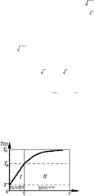
The second summand that is in square brackets of the expression (19) ranges from 0 to 1 and has almost zero influence on the temperature distribution in the frozen area. Therefore a linear temperature dependence can be employed which coincides with the solution of the stationary heat conductivity task in a flat one-layer wall with the width ξ changing over time. Fig. 2 shows a temperature distribution pattern in both phases.

I is the frozen soil for 0 z

II is the thawed soil for z

Fig. 2. Temperature distribution during freezing of the wet soil: z (t) for 0 z

21

Russian Journal of Building Construction and Architecture

Differentiating the expressions (18) and (19) using z and inserting the results into the Stefan conditions (4), we get the motion pseed of the freezing boundary

consisting of two summands. The second one is a dependence known from the automodel solutions [20]. The first summand describes the linear temperature distribution law along the frozen soil. If we assume that the initial temperature of the thawed soil is the same as the freezing one ТФ, the Stefan condition will be as follows [23]:

which is in keeping with the task of freezing the soil. Integration of the equation (21) yields a dependence of time on the freezing depth of the soil:

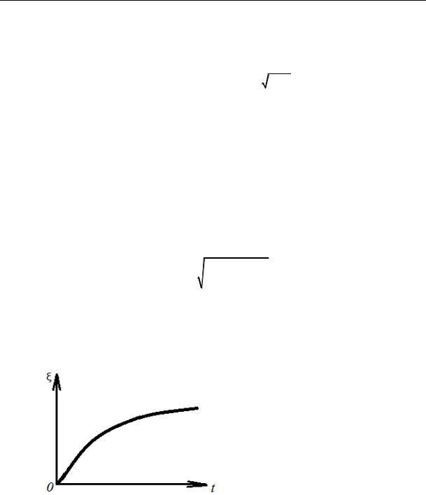
As can be seen, the growth rate of the frozen phase drops over time (Fig. 3). This might be due to an increase in the thermal resistance along with that in the freezing phase when the phase transition heat is depleted.

Fig. 3. Schematic of the growth

of the frozen area of the soil depending

on the time of freezing

Hence both components of the motion speed of the interphase boundary have the same time dependence and are in keeping with the data obtained for similar boundary problems regarding crystallization of other materials.

Conclusions. According to the study results, the following can be concluded.

1. An accurate analytical solution for the temperature distribution was obtained individually for the frozen and thawed area of the soil. This indicates the efficiency of the solution of the differential equations with particular derivates using the Laplace transform method.

22

2.An expression for the speed of motion of the freezing boundary of the wet soil was obtained consisting of two summands that have the same inverse dependence.

3.The temperature distribution in the frozen area does not have a linear dependence on the thickness of the freezing layer, which allows the results of stationary heat conductivity to be employed in similar tasks for heat transfer through a one-layer flat wall that changes its thickness over time.

4.The temperature field in the unfrozen wet soil complies with the known Gauss distribution and is in keeping with the previously obtained data.

5.The results can be also applied in designing as well as construction thermal physics, geophysics and metallurgy research.

References

1.Avdonin N. A. Matematicheskoe opisanie protsessov kristallizatsii [Mathematical description of crystallization processes]. Riga, Zinatne Publ., 1980. 180 p.

2.Bedrin E. A., Zav'yalov A. M., Zav'yalov M. A. Obespechenie termicheskoi ustoichivosti osnovaniya zemlyanogo polotna avtomobil'nykh dorog [Ensuring thermal stabilityof the roadbed base]. Omsk, 2012. 187 p.

3.Vasenin V. I. O zadache Stefana i raschetakh zatverdevaniya otlivok [On Stefan problem and the calculations of the solidification of castings]. Izvestiya Samarskogo nauchnogo tsentra RAN, 2012, vol. 14, no. 4 (5), pp. 1205—1211.

4.Vasil'ev V. I. Chislennoe reshenie promerzaniya grunta [Numerical solution of soil freezing]. Matematicheskoe modelirovanie, 2008, vol. 20, no. 7, pp. 119—124.

5.Veselov V. V., Belyakov V. A., Sal'nikov V. B. Reshenie nestatsionarnoi i nelineinoi teplovoi zadachi promerzaniya — ottaivaniya grunta metodom konechnykh elementov [Solution of non-stationary and nonlinear thermal problem of soil freezing — thawing byfinite element method]. Izvestiya vuzov. Stroitel'stvo, 2015, no. 2, pp. 95—99.

6.Ditkin V. A., Prudnikov A. P. Integral'nye preobrazovaniya i ischislenie [Integral transformations and calculus]. Moscow, Fizmatgiz Publ., 1961. 524 p.

7.Zav'yalov A. M., Bedrin E. A., Zav'yalov M. A. Apparat matematicheskogo modelirovaniya protsessov promerzaniya — protaivaniya gruntov [Apparatus of mathematical modeling of soil freezing — thawing processes]. Omskii nauchnyi vestnik, 2010, no. 3 (93), pp. 9—13.

8.Kudryavtsev V. A. Obshchee merzlotovedenie [General permafrost study]. Moscow, MGU Publ., 1978. 239 p.

9.Kumitskii B. M., Malyukov S. V., Savrasova N. A., Chuikin S. V. Primenenie usloviya Stefana dlya resheniya teplovykh zadach v ob"ektakh lesnogo kompleksa [The application of Stephan's condition for the solution of heat problems in the forest complex objects]. Lesotekhnicheskii zhurnal, 2017, vol. 7, no. 3 (27), pp. 41—48.

10.Kumitskii B. M., Savrasova N. A., Chernikov A. A. Raspredelenie temperatury v protsesse ostyvaniya odnorodnogo poluprostranstva [Temperature distribution during cooling of a homogeneous half-space].

Gradostroitel'stvo, infrastruktura, kommunikatsii, 2017, vol. 2 (7), pp. 28—33.

23

Russian Journal of Building Construction and Architecture

11.Maslov A. D., Osadchaya G. G., Tumel' N. V. e.a. Osnovy geokriologii [Basics of Geocryology]. Ukhta, IUIiB Publ., 2005. 176 p.

12.Meiramov A. M. Zadacha Stefana [Stefan problem]. Novosibirsk, Nauka Publ., 1986. 240 p.

13.Nagornova T. A. Matematicheskoe modelirovanie nasyshchennogo vlagoi grunta [Mathematical modeling of soil saturated with moisture]. Izvestiya Politekhnicheskogo un-ta, 2005, vol. 308, no. 6, pp. 126—129.

14.Osokin N. I., Sosnovskii A. V. Vliyanie dinamiki temperatury vozdukha i vysoty snezhnogo pokrova na promerzanie grunta [The influence of changes in air temperature and snow depth on soil freezing]. Kriosfera Zemli, 2015, vol. ХХI, no. 1, pp. 99—105.

15.Pavlov A. V. Teploobmen promerzayushchikh i protaivayushchikh gruntov s atmosferoi [Heat transfer and freezing prostaivaya soils with the atmosphere]. Moscow, Nauka Publ., 1965. 254 p.

16.Parfent'eva N. A., Samarin O. D. Zadacha Stefana v stroitel'stve [Stefan's task in construction]. Stroitel'nye materialy, oborudovanie, tekhnologii ХХI veka. — 2002. —№ 6. — S. 34—37.

17.Parfent'eva N. A. Matematicheskoe modelirovanie teplovogo rezhima konstruktsii pri fazovykh perekhodakh [Mathematical modeling of thermal regime of structures at phase transitions]. Vestnik MGSU, 2011, no. 4, pp. 340—345.

18.Parfent'eva N. A., Samarin O. D., Kashintseva V. L. O primenenii i reshenii zadachi Stefana v stroitel'noi teplofizike [On the application and solution of the Stefan problem in building thermal physics]. Vestnik MGSU, 2011, no. 4, pp. 323—328.

19.Rubinshtein L. I. Problema Stefana [Stefan's Problem]. Riga, Zvaigne Publ., 1967. 458 p.

20.Tikhonov A. N., Samarskii A. A. Uravneniya matematicheskoi fiziki [Equations of mathematical physics]. Moscow, Izd-vo MGU, 2004. 798 p.

21.Fel'dman G. M. Metody rascheta temperaturnogo rezhima merzlykh gruntov [Methods of calculating the temperatureregime of frozen soils]. Moscow, Nauka Publ., 1973. 254 p.

22.Fikhtengol'ts G. M. Kurs differentsial'nogo i integral'nogo ischisleniya [Course of differential and integral calculus]. Moscow, Fizmatlit Publ., 2001. 663 p.

23.Tsaplin A. I., Nikulin I. L. Modelirovanie teplofizicheskikh protsessov i ob"ektov v metallurgii [Modeling of thermophysical processes and objects in metallurgy]. Perm', Izd-vo Permskogo gos. un-ta, 2011. 299 p.

24.Tsytovich N. A. Mekhanika merzlykh gruntov [Mechanics of frozen soils]. Moscow, Vyssh. shk. Publ., 1973. 448 p.

25.Clapeyron B. P. Theorie mecanique de la chaleur. Paris, Gauthier-Villars, 1883. 347 р.

26.Crank J. Free and Moving BoundaryProblems. Oxford, Clarendon Press, 1984. 425 p.

27.Lame G., Clapeyron B. P. Memorie sur colidification par refroidissiment d`un globe liguide. Annales de Chimie et de Physigue, 1831, vol. 47, pp. 250—256.

28.Ruddle R. W. The Solidification of Castings. London, The Inst. of Metals, 1957. 391 p.

29.Stefan J. Ubereinige Probleme der Theorie der Warmeletung. Sitzungsberichte der kaiserliche Akademie der Wissenschaften in Wien, 1889, Bd. XCVIII, pp. 473—484.

24

DOI 10.25987/VSTU.2019.42.2.003

UDC 517.95 : 536.4

А. S. Ryabenko1, S. N. Kuznetsov2

DETERMINING THE TEMPERATURE IN A SEMIPLANE

WITH A SLANT LINEAR CRACK REACHING THE HALF PLANE BOUNDARY

Voronezh State University

Russia, Voronezh, e-mail: alexr-83@yandex.ru

1PhD in Physics and Mathematics, Assoc. Prof. of the Dept. of Equations

in Particular Derivatives and Probability Theories

Voronezh State Technical University

Russia, Voronezh, tel.: (473)271-53-21, e-mail: teplosnab_kaf@vgasu.vrn.ru

2D. Sc. In Engineering, Assoc. Prof., Prof. of the Dept. of Heat and Gas Supply and Oil and Gas Business

Statement of the problem. The paper looks at temperatures in a homogeneous half plane with a finite rectangular crack reaching the half plane boundary on the condition that the temperature at the half plane boundaryas well as temperature and heat flow fluctuations in the crack are known.

Results. A mathematical model is suggested that describes a stationary heat distribution in a homogeneous half plane with a linear crack reaching the half plane boundary for when the temperature at the half plane as well as temperature and heat flow fluctuations in the crack are known. The model was proved to be mathematically correct and the method of designing it as well as a whole range of related tasks was presented. The formula for presenting the solution ofthemodel was obtained.

Conclusions. The resulting formula can be employed to study the temperature distribution in a material experiencing cracking as well as in adjacent areas in order to evaluate its effect on heat distribution.

Keywords: temperature, crack, heat flow, heat distribution, equation of stationary heat conductivity.

Introduction. The problem of mathematical description of physical characteristics of materials and defected structures is rather complex and multifaceted (see [6], [7], [12], [17], [18]). This is due to a great variety of materials, structure shapes, types and geometries of defects. One of the aspects of mathematical description of materials and defected structures is to study thermal processes occurring in them(see [3]––[5], [8]––[11], [13]––[16]).

© Ryabenko А. S., Kuznetsov S. N., 2019

25

Russian Journal of Building Construction and Architecture

Cracks and other defects cause extra redistribution of heat flows and thus extra strains. Therefore mathematical models describing heat distribution in defected materials and structures can shed some light on the effect of defects on heat flows and temperature distribution.

The paper sets forth a mathematical model for describing heat distribution in a homogeneous half plane with a linear crack to an angle to the half plane boundary. This article is a followup of [3], [8], [9], [13] where heat distribution in functional and gradient materials with internal cracking has been investigated. Special attention is paid to proving that the suggested model is mathematically correct as unless it is, the outcome might not relate to the model and only to certain oftentimes rigid input data requirements.

1. Statement of the problem. Major denotations. Let be a fixed angle in the range of 0 to 180 degrees, n is a vector with the coordinates( sin ;cos ).

Let us introduce the denotations: 2 x 2 | x1 , x2 0 is the upper half plane, l x 2 | x1 tcos , x2 tsin , where t (0;|l |) is the interval in the upper half plane

reaching the half plane boundary, l is a line corresponding to l .

The task (1.1)––(1.4) describes a stationary heat distribution in the upper half plane with a cut in the line l reaching the half plane boundary under the angle . The line l models cracking. The equation (1.1) was obtained using the equation of stationary heat distribution in a sold body with no heat sources div(k(x)gradu(x)) 0 where k(x) is the coefficient of internal heat conductivity, at k(x) const 0. The function u(x) determines the temperature at

26

the point x. The condition (1.2) specifies the temperature at the half plane boundary and the conditions (1.3) and (1.4) specify a temperature and heat flow fluctuation in the crack l respectively.

The conditions (1.3) and (1.4) are interpreted as follows:

u(x 0 n) u(x 0 n) lim(u(x n) u(x n)),

0

sical solution of the equation (1.1) for which the extra conditions (1.2), (1.3) and (1.4) are met.

2. Reducing to the generalized equation. Let 2 x 2 | x1 , x2 0 denote the lower half plane, l x 2 | x1 tcos , x2 tsin ,where t (0;|l |) denote the interval in the

lower half plane reaching the half plane boundary, l denotes a line corresponding to l . Let us assume that the task (1.1)-(1.4) has a solution.

Let us look at the function

27

Russian Journal of Building Construction and Architecture

Based on (1.3), at t 0;|l | .

Calculating the generalized derivatives from the function u(x) in a traditional way conside-

28

3. Designing the solutions for the generalized equation. In 2 a fundamental solution of

the Laplace operator is the function 1 ln x (see [2]), then the solution of the equation (2.6) 2

is given by the formula

where is used for a convolution of the generalized functions (see [1]).

Using the properties of the convolutions of the generalized functions (see[1]), we get that

As l contains the support of the generalized function q(x) l (x), for any main function (x) fromD( 2 )

where (x) is a random function from D( 2 ) that is such that (x) 1 in the vicinity of l(see [1]). Determining the direct product of the generalized functions (see [1]) we see that