

755
.pdf74 |
3G Evolution: HSPA and LTE for Mobile Broadband |
Frequency |
Frequency |
Time |
Time |
(a) |
(b) |
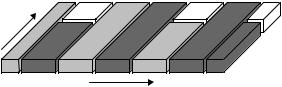
Figure 5.6 Orthogonal multiple access: (a) TDMA and (b) FDMA.
Mutually orthogonal uplink transmissions within a cell can be achieved in the time domain (Time Division Multiple Access, TDMA), as illustrated in Figure 5.6a. TDMA implies that different mobile terminals within in a cell transmit in different non-overlapping time intervals. In each such time interval, the full system bandwidth is then assigned for uplink transmission from a single mobile terminal.
Alternatively, mutually orthogonal uplink transmissions within a cell can be achieved in the frequency domain (Frequency Division Multiple Access, FDMA) as illustrated in Figure 5.6b, that is by having mobile terminals transmit in different frequency bands.
To be able to provide high-rate packet-data transmission, it should be possible to assign the entire system bandwidth for transmission from a single mobile terminal. At the same time, due to the burstiness of most packet-data services, in many cases mobile terminals will have no uplink data to transmit. Thus, for efficient packet-data access, a TDMA component should always be part of the uplink multiple-access scheme.
However, relying on only TDMA to provide orthogonality between uplink transmissions within a cell could be bandwidth inefficient, especially in case of a very wide overall system bandwidth. As discussed in Chapter 3, a wide bandwidth is needed to support high data rates in a power-efficient way. However, the data rates that can be achieved over a radio link are, in many cases, limited by the available signal power (power-limited operation) rather than by the available bandwidth. This is especially the case for the uplink, due to the, in general, more limited mobile-terminal transmit power. Allocating the entire system bandwidth to a single mobile terminal could, in such cases, be highly inefficient in terms of bandwidth utilization. As an example, allocating 20 MHz of transmission bandwidth to a mobile terminal in a scenario where the achievable uplink data rate, due to mobile-terminal transmit-power limitations, is anyway limited to, for example, a few 100 kbps would obviously imply a very inefficient usage of the overall available bandwidth. In such cases, a smaller transmission bandwidth should be
Wider-band ‘single-carrier’ transmission |
75 |
Frequency |
|
Time
Figure 5.7 FDMA with flexible bandwidth assignment.
assigned to the mobile terminal and the remaining part of the overall system bandwidth should be used for uplink transmissions from other mobile terminals. Thus, in addition to TDMA, an uplink transmission scheme should preferably allow for orthogonal user multiplexing also in the frequency domain, i.e. FDMA.
At the same time, it should be possible to allocate the entire overall transmission bandwidth to a single mobile terminal when the channel conditions are such that the wide bandwidth can be efficiently utilized, that is when the achievable data rates are not power limited. Thus an orthogonal uplink transmission scheme should allow for FDMA with flexible bandwidth assignment as illustrated in Figure 5.7.
Flexible bandwidth assignment is straightforward to achieve with an OFDM-based uplink transmission scheme by dynamically allocating different number of subcarriers to different mobile terminals depending on their instantaneous channel conditions. In the next section, it will be discussed how this can also be achieved in case of low-PAR ‘single-carrier’ transmission, more specifically by means of so-called DFT-spread OFDM.
5.3 DFT-spread OFDM
DFT-spread OFDM (DFTS-OFDM) is a transmission scheme that can combine the desired properties discussed in the previous sections, i.e.:
•Small variations in the instantaneous power of the transmitted signal (‘singlecarrier’ property).
•Possibility for low-complexity high-quality equalization in the frequency domain.
•Possibility for FDMA with flexible bandwidth assignment.
Due to these properties, DFTS-OFDM has been selected as the uplink transmission scheme for LTE, that is the long-term 3G evolution, see further Part IV of this book.
5.3.1 Basic principles
The basic principle of DFTS-OFDM transmission is illustrated in Figure 5.8. Similar to OFDM modulation, DFTS-OFDM relies on block-based signal generation.
76 |
|
|
|
|
|
|
|
3G Evolution: HSPA and LTE for Mobile Broadband |
||||||||||
|
|
|
|
|
|
|
|
|
|
|
|
|
|
|
|
|
|
|
|
|
Transmitter |
|
|
|
|
|
|
|
|
|
|
|
|
|
|
|
|
|
|
|
|
|
|
0 |
|
|
|
|
|
|
|
|
|
|
|
|
|
|
|
|
|
|
|
|
|
|
|
|
|
|
|
|
|
|
|
|
|
|
|
|
|
|
|
|
|
|
|
|
|
|
|
|
|
|
|
a0, a1, ..., aM 1 |
|
|
|
|
|
|
|
|
|
|
|
|
|
x(t) |
|||
|
|
|
|
|
|
|
|
|
|
|
|
|
|
|||||
|
|
Size-M |
|
|
|
Size-N |
|
|
|
|
|
|
|
|||||
|
|
|
|
|
|
|
|
|
|
|
|
|||||||
|
|
|
|
|
|
|
|
|
|
|
|
|||||||
|
|
|
|
|
|
CP |
D/A conversion |
|||||||||||
|
|
|
|
|
DFT |
|
|
|
IDFT |
|
|
|
|
|
|
|
||
|
|
|
|
|
|
|
|
|
|
|
|
|
|
|
|
|
||
|
|
|
|
|
|
|
|
|
|
|
|
|
|
|
|
|
|
|
|
|
|
|
|
|
|
|
|
|
|
|
|
|
|
|
|
|
|
|
|
|
|
|
|
|
|
|
|
|
|
|
|
|
|
|
|
|
M 0
N
Figure 5.8 DFTS-OFDM signal generation.
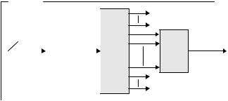
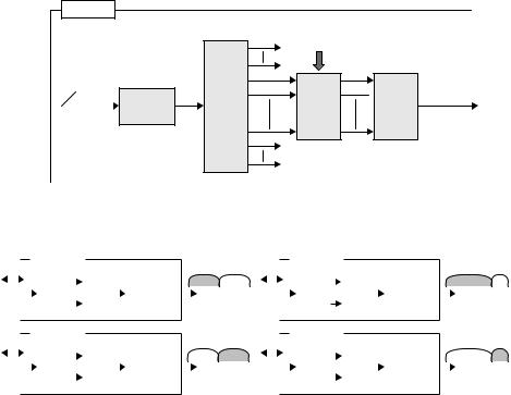
In case of DFTS-OFDM, a block of M modulation symbols from some modulation alphabet, e.g. QPSK or 16QAM, is first applied to a size-M DFT. The output of the DFT is then applied to consecutive inputs of a size-N inverse DFT where N > M and where the unused inputs of the IDFT are set to zero. Typically, the inverseDFT size N is selected as N = 2n for some integer n to allow for the IDFT to be implemented by means of computationally efficient radix-2 IFFT. Also similar to OFDM, a cyclic prefix is preferable inserted for each transmitted block. As discussed in Section 5.1.2, the presence of a cyclic prefix allows for straightforward low-complexity frequency-domain equalization at the receiver side.
Comparing Figure 5.8 with the IFFT-based implementation of OFDM modulation it is obvious that DFTS-OFDM can alternatively be seen as OFDM modulation preceded by a DFT operation, i.e. pre-coded OFDM.
If the DFT size M would equal the IDFT size N, the cascaded DFT and IDFT blocks of Figure 5.8 would completely cancel out each other. However, if M is smaller than N and the remaining inputs to the IDFT are set to zero, the output of the IDFT will be a signal with ‘single-carrier’ properties, i.e. a signal with low power variations, and with a bandwidth that depends on M. More specifically, assuming a sampling rate fs at the output of the IDFT, the nominal bandwidth of the transmitted signal will be BW = M/N · fs. Thus, by varying the block size M the instantaneous bandwidth of the transmitted signal can be varied, allowing for flexible-bandwidth assignment. Furthermore, by shifting the IDFT inputs to which the DFT outputs are mapped, the transmitted signal can be shifted in the frequency domain, as will be further discussed in Section 5.3.3.
To have a high degree of flexibility in the instantaneous bandwidth, given by the DFT size M, it is typically not possible to ensure that M can be expressed as 2m for some integer m. However, as long as M can be expressed as a product of relatively small prime numbers, the DFT can still be implemented as relatively
Wider-band ‘single-carrier’ transmission |
|
|
|
|||||
|
1 |
|
|
|
|
|
|
|
x} |
0.1 |
|
|
|
|
|
|
|
{PAR |
|
|
|
|
DFTS-OFDM |
OFDM |
||
Prob |
0.01 |
|
|
|
||||
|
|
|
|
|
|
|
||
|
|
|
|
|
|
|
|
|
|
0.001 |
|
|
|
|
|
|
|
|
5 |
6 |
7 |
8 |
9 |
10 |
11 |
12 |
77
Cubic metric:
-OFDM: 3.4dB
-DFTS-OFDM (QPSK): 1.0dB
-DFTS-OFDM (16QAM): 1.8dB
x (dB)
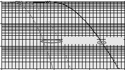
Figure 5.9 PAR distribution for OFDM and DFTS-OFDM, respectively. Solid curve: QPSK. Dashed curve: 16QAM.
low-complexity non-radix-2 FFT processing. As an example, a DFT size M = 144 can be implemented by means of a combination of radix-2 and radix-3 FFT processing (144 = 32 · 24).
The main benefit of DFTS-OFDM, compared to a multi-carrier transmission scheme such as OFDM, is reduced variations in the instantaneous transmit power, implying the possibility for increased power-amplifier efficiency. This benefit of DFTS-OFDM is illustrated in Figure 5.9, which illustrates the distribution of the Peak-to-Average-power Ratio (PAR) for DFTS-OFDM and conventional OFDM. The PAR is defined as the peak power within one IDFT block (one OFDM symbol) normalized by the average signal power. It should be noted that the PAR distribution is not the same as the distribution of the instantaneous transmit power as illustrated in Figure 3.3. Historically, PAR distributions have often been used to illustrate the power variations of OFDM.
As can be seen in Figure 5.9, the PAR is significantly lower for DFTS-OFDM, compared to OFDM. In case of 16QAM modulation, the PAR of DFTS-OFDM increases somewhat as expected (compare Figure 3.3). On the other hand, in case of OFDM the PAR distribution is more or less independent of the modulation scheme. The reason is that, as the transmitted OFDM signal is the sum of a large number of independently modulated subcarriers, the instantaneous power has an approximately exponential distribution, regardless of the modulation scheme applied to the different subcarriers.
Although the PAR distribution can be used to qualitatively illustrate the difference in power variations between different transmission schemes, it is not a very good measure to more accurately quantify the impact of the power variations on e.g. the required power-amplifier back-off.
78 |
3G Evolution: HSPA and LTE for Mobile Broadband |
|
Receiver |
|
|
|
|
|
|
|
|
|
|
|
|
|
|
r(t) |
|
rn |
|
|
|
|
Size-N |
|
|
|
|
|
|||
|
|
CP |
|
|
|||
|
|
|
|
removal |
|
|
DFT |
|
|
|
|
|
|
|
|
|
|
|
|
|
|
|
|
Discard |
|
Size-M |
aˆ0, aˆ1, ..., aˆM 1 |
IDFT |
|
Discard |
|
Figure 5.10 Basic principle of DFTS-OFDM demodulation.
A better measure of the impact on the required power-amplifier back-off and the corresponding impact on the power-amplifier efficiency is given by the so-called cubic metric [49]. The cubic metric is a measure of the amount of additional backoff needed for a certain signal wave form, relative to the back-off needed for some reference wave form.
As can be seen from Figure 5.9, the cubic metric (given to the right of the graph) follows the same trend as the PAR. However, the differences in cubic metric are somewhat smaller than the corresponding differences in PAR.
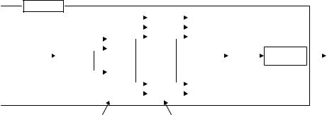
5.3.2DFTS-OFDM receiver
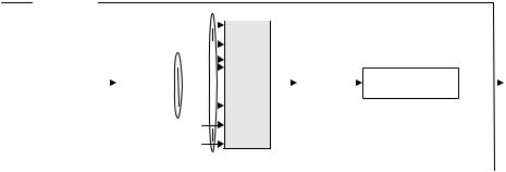
The basic principle of demodulation of a DFTS-OFDM signal is illustrated in Figure 5.10. The operations are basically the reverse of those for the DFTS-OFDM signal generation of Figure 5.8, i.e. size-N DFT (FFT) processing, removal of the frequency samples not corresponding to the signal to be received, and size-M inverse DFT processing.
In the ideal case with no signal corruption on the radio channel, DFTS-OFDM demodulation according to Figure 5.10 will perfectly restore the block of transmitted symbols. However, in case of a time dispersive or, equivalently, a frequency-selective radio channel, the DFTS-OFDM signal will be corrupted, with ‘self-interference’ as a consequence. This can be understood in two ways:
1.Being a wideband single-carrier signal, the DFTS-OFDM spread signal is, obviously, corrupted in case of a time-dispersive channel.
2.If the channel is frequency selective over the span of the DFT, the inverse DFT at the receiver will not be able to correctly reconstruct the original block of transmitted symbols.
Wider-band ‘single-carrier’ transmission |
79 |
Receiver
r(t) |
|
rn |
CP |
removal
|
Frequency-domain |
|
|
equalization |
|
Size-N |
W |
|
DFT |
||
|
 Size-M aˆ0, aˆ1, ..., aˆM 1
IDFT
Figure 5.11 DFTS-OFDM demodulator with frequency-domain equalization.
|
|
|
|
|
Terminal A |
|
|
|
|
|
|
|
|
|
|
|
|
|
Terminal A |
|
|
|
|
|
|
|
|
|||||||
|
M1 |
|
|
|
|
|
|
|
|
|
|
|
|
M1 |
|
|
|
|
|
|
|
|
||||||||||||
|
|
|
|
|
|
|
|
|
|
|
|
|
|
|
|
|
|
|
|
|
|
|
|
|
|
|
|
|
|
|
|
|
|
|
|
|
|
|
|
DFT |
|
|
|
IDFT |
|
|
Additional |
|
|
|
|
|
|
|
|
|
DFT |
|
|
|
IDFT |
|
|
Additional |
|
|
|
|
|
|
|
|
|
|
(M) |
0 |
|
|
|
|
processing |
|
|
|
|
|
|
|
|
|
(M1) |
|
|
|
|
|
|
processing |
|
|
|
|
||
|
|
|
|
|
|
|
|
|
|
|
|
|
|
|
|
|
|
|
|
|
|
|
|
|
|
|
|
|||||||
|
|
|
|
|
|
|
|
|
|
|
|
|
|
|
|
|
|
|
|
|
|
|
|
|
|
|
|
|
|
|||||
|
|
|
|
|
|
|
|
|
|
|
|
|
|
|
|
|
|
|
|
|
|
|
|
|
|
|||||||||
|
|
|
|
|
Terminal B |
|
|
|
|
|
|
|
|
|
|
|
|
|
Terminal B |
|
|
|
|
|
|
|
|
|||||||
|
M2 |
|
|
|
|
|
|
|
|
|
|
|
|
M2 |
|
|
|
|
|
|
|
|
||||||||||||
|
|
|
|
|
|
0 |
|
|
|
|
|
|
|
|
|
|
|
|
|
|
|
|
0 |
|
|
|
|
|
|
|
|
|
|
|
|
|
|
|
|
DFT |
|
|
IDFT |
|
|
Additional |
|
|
|
|
|
|
DFT |
|
|
IDFT |
|
|
Additional |
|
|
|
|
||||||
|
|
|
|
|
|
|
|
|
|
|
|
|
|
|
|
|
|
|
|
|||||||||||||||
|
|
|
|
|
(M) |
|
|
|
|
|
|
processing |
|
|
|
|
|
|
|
|
|
(M2) |
|
|
|
|
|
|
|
processing |
|
|
|
|
|
|
|
|
|
|
|
|
|
|
|
|
|
|
|
|
|
|
|
|
|
|
|
|
|
|
|
|
|
|
|
|
|
|
|
|
|
|
|
|
M1 M2 |
|
|
|
|
|
|
|
|
|
|
|
|
|
M1 M2 |
|
|
|
|
|
|
|
|
|||||||
|
|
|
|
|
|
|
|
|
|
(a) |
|
|
|
|
|
|
|
|
|
|
|
|
|
|
|
(b) |
|
|
|
|
||||
Figure 5.12 Uplink user multiplexing in case of DFTS-OFDM. (a) Equal-bandwidth assignment and (b) unequal-bandwidth assignment.
Thus, in case of DFTS-OFDM, an equalizer is needed to compensate for the radiochannel frequency selectivity. Assuming the basic DFTS-OFDM demodulator structure according to Figure 5.10, frequency-domain equalization as discussed in Section 5.1.2 is especially applicable to DFTS-OFDM transmission (see Figure 5.11).
5.3.3 User multiplexing with DFTS-OFDM
As mentioned above, by dynamically adjusting the transmitter DFT size and, consequently, also the size of the block of modulation symbols a0, a1, . . . , aM−1, the nominal bandwidth of the DFTS-OFDM signal can be dynamically adjusted. Furthermore, by shifting the IDFT inputs to which the DFT outputs are mapped, the exact frequency-domain ‘position’ of the signal to be transmitted can be adjusted. By these means, DFTS-OFDM allows for uplink FDMA with flexible bandwidth assignment as illustrated in Figure 5.12.
80 |
3G Evolution: HSPA and LTE for Mobile Broadband |
Transmitter
a0, a1, ... , aM 1 |
|
|
|
|
|
|
|
|
|
|
|
|
|
|
|
|
x(t) |
|
|
|
|
|
|
|
|
|
|
|
|
|
|
|
|
|
|||
|
|
|
|
|
|
|
|
|
|
|
|
|
|
|
|
|||
Size-M |
|
|
BW. |
|
|
|
|
|
Size-N |
|
|
|
|
|
|
|||
|
|
|
|
|
|
|
|
|
|
|
|
|
||||||
|
|
|
|
P |
|
|
|
|
|
|
|
D/A |
||||||
|
|
|
|
|
|
|
|
CP |
||||||||||
|
|
DFT |
|
|
exp. |
|
|
|
|
IDFT |
|
|
|
|
conversion |
|
||
|
|
|
|
|
|
|
|
|
|
|
|
|
|
|
|
|
|
|
|
|
|
|
|
|
|
|
|
|
|
|
|
|
|
|
|
|
|
|
|
|
|
|
|
|
|
|
|
|
|
|
|
|
|
|
|
|
|
|
|
|
|
|
|
|
|
|
|
|
|
|
|
|
|
|
|
|
|
|
|
|
|
|
|
|
|
|
|
|
|
|
|
|
|
|
Bandwidth |
Spectrum |
expansion |
shaping |
Figure 5.13 DFTS-OFDM with frequency-domain spectrum shaping.
Figure 5.12a illustrates the case of multiplexing the transmissions from two mobile terminals with equal bandwidth assignments, that is equal DFT sizes M, while Figure 5.12b illustrates the case of differently sized bandwidth assignments.
5.3.4DFTS-OFDM with spectrum shaping
DFTS-OFDM signal generation according to Figure 5.8 corresponds to a signal with a rectangular-shaped spectrum. To further reduce the power variations of the DFTS-OFDM signal, explicit spectrum shaping can be applied. This is similar to the spectrum shaping applied to, for example, a WCDMA signal, as described in Chapter 3 (Figure 3.6).
Spectrum shaping for DFTS-OFDM is illustrated in Figure 5.13. After size-M DFT processing of the block of modulation symbols, the signal is periodically expanded in the frequency domain. Spectrum shaping is then applied by multiplying the frequency samples with some spectrum-shaping function, e.g. a root-raised-cosine function (raised-cosine-shaped power spectrum). The signal is then transformed back to the time domain by means of the size-N IDFT/IFFT.
As shown in Figure 5.14, spectrum shaping allows for further reduction in the power variations of the transmitted signal, thus allowing for even higher poweramplifier efficiency. The cost of spectrum shaping is reduced spectrum efficiency as the spectrum shaping implies a wider spectrum for the same DFT-size M. As an example, a roll-off α = 0.22 implies 22% excess bandwidth, compared to no spectrum shaping. Spectrum shaping should thus only be applied to power-limited scenarios where transmit power, rather than spectrum, is the scarce resource. The reduced power variations due to spectrum shaping can then be used to further improve, for example, uplink coverage.
Wider-band ‘single-carrier’ transmission |
|
|
|
81 |
|||||
|
1 |
|
|
|
|
|
|
|
Cubic metric: |
|
|
|
|
|
|
|
|
|
|
|
|
|
|
|
|
|
|
|
- OFDM: 3.4 dB |
} |
|
|
|
|
|
|
|
|
- DFTS-OFDM (a 0.0): 1.0 dB |
x |
|
|
|
|
DFTS-OFDM |
|
|
||
0.1 |
|
|
|
|
|
- DFTS-OFDM (a 0.15): 0.6 dB |
|||
|
|
|
|
|
|
||||
|
|
|
|
|
|
|
|
- DFTS-OFDM (a 0.22): 0.45 dB |
|
{PAR |
|
|
|
|
|
|
|
|
|
a 0.22 |
a 0.15 |
a 0 |
|
|
OFDM |
||||
Prob |
|
|
|||||||
0.01 |
|
|
|
|
|
|
|
|
|
|
|
|
|
|
|
|
|
|
|
|
0.001 |
|
|
|
|
|
|
|
|
|
4 |
5 |
6 |
7 |
8 |
9 |
10 |
11 |
12 |
|
|
|
|
|
x (dB) |
|
|
|
|
Figure 5.14 PAR distribution and cubic metric for DFTS-OFDM with different spectrum shaping.
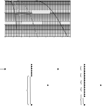
Localized DFT-S-OFDM |
|
|
|
|
Distributed DFT-S-OFDM |
|
|||||||||||||
|
|
|
|
|
|
|
|
|
|
|
|
|
|
|
|
|
|
|
|
Size-M |
|
|
|
|
|
|
|
|
|
Size-M |
|
|
|
|
0 |
|
|
|
|
|
|
|
|
|
|
|
|
|
|
|
|
|
|
||||||
DFT |
|
|
|
|
|
|
|
|
|
DFT |
|
|
|
|
|
|
|||
|
|
|
|
|
|
|
|
|
|
|
|
|
|
0 |
|
|
|
|
|
|
|
|
|
|
|
|
|
|
|
|
|
|
|
|
|
|
|
||
M 5 |
|
|
|
|
|
M 5 |
|
|
|||||||||||
|
|
|
|
|
|
|
|
|
|
|
|
|
|
||||||
|
|
|
|
|
Size-N |
|
|
|
|
|
|
|
0 |
|
|
Size-N |
|
||
|
|
|
|
|
|
|
|
|
|
|
|
|
|
|
|||||
|
|
|
|
|
|
|
|
|
|
|
|
|
|
|
|||||
|
|
|
|
|
|
|
|
|
|
|
|
|
|
|
|
|
|
||
|
|
|
|
|
IDFT |
|
|
|
|
|
|
|
|
|
|
|
|
IDFT |
|
0 |
|
|
|
|
|
|
|
|
|
0 |
|
|
|
||||||
|
|
|
|
|
|
|
|
|
|
|
|
||||||||
|
|
|
|
|
|
|
|
|
|
|
|
|
|
||||||
|
|
|
|
|
|
|
|
|
|
|
|
|
|
||||||
|
|
|
|
|
|
|
|
|
|
|
|
|
|
|
|
|
|
||
|
|
|
|
|
|
|
|
|
|
|
|
|
|
|
|
|
|
|
|
|
|
|
|
|
|
|
|
|
|
|
0 |
|
|
|
|
||||
|
|
|
|
|
|
|
|
|
|
|
|
|
|
|
|||||
|
|
|
|
|
|
|
|
|
|
|
|
|
|
|
|||||
|
|
|
|
|
|
|
|
|
|
|
|
|
|
|
|
|
|
|
|
|
|
|
|
|
|
|
|
|
|
|
|
|
|
|
|
|
|
|
|
|
(a) |
|
|
|
|
|
|
|
|
(b) |
|
|
|||||||
Figure 5.15 Localized DFTS-OFDM vs. Distributed DFTS-OFDM.
5.3.5 Distributed DFTS-OFDM
What has been illustrated in Figure 5.8 can more specifically be referred to as Localized DFTS-OFDM, referring to the fact that the output of the DFT is mapped to consecutive inputs of the IFFT. An alternative is to map the output of the DFT to equidistant inputs of the IDFT with zeros inserted in between, as illustrated in Figure 5.15. This is can also be referred to as Distributed DFTS-OFDM.
Figure 5.16 illustrates the basic structure of the transmitted spectrum in case of localized and distributed DFTS-OFDM, respectively. Although the spectrum of the localized DFTS-OFDM signal clearly indicates a single-carrier transmission this is not as clearly seen from the spectrum of the distributed DFTS-OFDM signal. However, it can be shown that a distributed DFTS-OFDM signal has similar power variations as localized DFTS-OFDM. Actually, it can be shown that a distributed DFTS-OFDM signal is equivalent to so-called Interleaved FDMA (IFDMA) [67].
82 |
|
3G Evolution: HSPA and LTE for Mobile Broadband |
||||
|
|
|
|
|
|
|
|
|
|
|
|
|
|
Localized transmission |
Distributed transmission |
(a) |
(b) |
Figure 5.16 Spectrum of localized and distributed DFTS-OFDM signals.
|
|
|
|
|
|
|
|
|
|
|
Localized transmission |
|
|
Distributed transmission |
|||
|
|
|
(a) |
|
|
(b) |
||
Figure 5.17 User multiplexing in case of localized and distributed DFTS-OFDM.
The benefit of distributed DFTS-OFDM, compared to localized DFTS-OFDM, is the possibility for additional frequency diversity as even a low-rate distributed DFTS-OFDM signal (small DFT size M) can be spread over a potentially very large overall transmission bandwidth.
User multiplexing in the frequency domain as well as flexible bandwidth allocation is possible also in case of distributed DFTS-OFDM. However, in this case, the different users are ‘interleaved in the frequency domain, as illustrated in Figure 5.17b (thus the alternative term “Interleaved FDMA”)’. As a consequence, distributed DFTS-OFDM is more sensitivity to frequency errors and has higher requirements on power control, compared to localized DFTS-OFDM. This is similar to the case of localized OFDM vs. distributed OFDM as discussed in Section 4.10.
6
Multi-antenna techniques
Multi-antenna techniques can be seen as a joint name for a set of techniques with the common theme that they rely on the use of multiple antennas at the receiver and/or the transmitter, in combination with more or less advanced signal processing. Multi-antenna techniques can be used to achieve improved system performance, including improved system capacity (more users per cell) and improved coverage (possibility for larger cells), as well as improved service provisioning, for example, higher per-user data rates. This chapter will provide a general overview of different multi-antenna techniques applicable to the 3G evolution. How multiantenna techniques are specifically applied to HSPA and its evolution and to LTE is discussed in somewhat more details in Part III and IV, respectively.
6.1 Multi-antenna configurations
An important characteristic of any multi-antenna configuration is the distance between the different antenna elements, to a large extent due to the relation between the antenna distance and the mutual correlation between the radio-channel fading experienced by the signals at the different antennas.
The antennas in a multi-antenna configuration can be located relatively far from each other, typically implying a relatively low mutual correlation. Alternatively, the antennas can be located relatively close to each other, typically implying a high mutual fading correlation, that is in essence that the different antennas experience the same, or at least very similar, instantaneous fading. Whether high or low correlation is desirable depends on what is to be achieved with the multi-antenna configuration (diversity, beam-forming, or spatial multiplexing) as discussed further below.
What actual antenna distance is needed for low, alternatively high, fading correlation depends on the wavelength or, equivalently, the carrier frequency used for the radio communication. However, it also depends on the deployment scenario.
83