

76
.pdfResearch of the stress state of an element of a thick-wall pipeline . . . |
111 |
mechanochemical corrosion in the framework of the linear theory of elasticity is given in [9]. Moreover, the process of metal loss is significantly extended over time. In case of intergranular and transcrystalline corrosion, on the contrary, the mechanical properties of the metal change practically without loss of its weight [8]. The combined action of corrosion and static tensile stresses leads to a gradual decrease in the resistance to plastic deformation and a decrease in the plasticity limit in ductile metals, carbon and low alloy steels, and various alloys [10]. The decrease in the mechanical properties of the material during loading due to the accumulation of damage and defects can be taken into account in the framework of the plasticity theory of inhomogeneous bodies [11, 12, 13]. In [11, 12, 13], to take into account the accumulation of damage to the material, it was proposed to introduce a special softening function (radial inhomogeneity of strength characteristics) in the criteria used for plasticity of the material for axisymmetric and some plane problems. In [14], modified plasticity criteria were used, which can take into account the accumulation of material damage in the case of more complex boundary conditions under which plastic inhomogeneity should change in accordance with the change in the elastoplastic boundary. In this paper, this is exactly the approach taken.
3 Solution of the problem
3.1 Basic assumptions and relationships
The element of a thick-walled extended pipeline is in flat deformation conditions. Consider the cross section of a pipeline with an internal circuit a0 + f1(r, θ) and an external circuit 1 + f2(r, θ) in the polar coordinate system r, θ. The material of the pipeline is considered perfectly elastic-plastic.
The equations of equilibrium of the pipeline have the form:
∂σr |
+ |
1 |
|
∂τrθ |
+ |
σr − σθ |
= 0, |
∂τrθ |
+ |
1 ∂σθ |
+ 2 |
τrθ |
= 0. |
(1) |
||||
|
|
|
|
|
|
|
|
|
|
|
||||||||
∂r |
|
r |
|
∂θ |
r |
∂r |
|
r ∂θ |
r |
|||||||||
|
|
|
|
|
|
|
|
|
|
|||||||||
Here are σr, σθ, τrθ the components of the stress tensor. In the elastic region, Hooke’s law is valid for a homogeneous, isotropic linearly elastic material:
εij = |
1 |
((1 + μ)σij − μδijσkk). |
(2) |
E |
Where σij and εij are the components of the stress and strain tensors, E – is the elastic modulus, μ – is the Poisson’s ratio, δij – is the Kronecker symbol.
As a condition for the transition of the material into a plastic state, we accept the Tresca- Saint-Venant condition, which is widely used in the calculation of plastic deformable metal structures
(σθ − σr)2 + 4τrθ2 = 4K2 |
(3) |
where K is adhesion coe cient.
The material strength parameter K in condition (2) characterizes the plastic inhomogeneity formed as a result of varying degrees of damage to the material due to the force-corrosion e ect and distributed over the thickness of the plastic zone, similar to the outline of its boundary. At the boundary of the plastic zone, the value K is constant: K = K1. The value

112 A.M. Alimzhanov, K.Zh. Shetiyeva
K is a special softening function, depending on the coordinates r, θ and loading parameters r0, δ [14]:
K = K (r, r0, θ, δ) |
(4) |
Here r0, δ – is the axisymmetric and nonaxisymmetric loading parameters: r0 = r0(P0, P1 +
P2), δ = δ(P1 − P2).
The problem is solved by the method of joint use of static and physical equations for the considered elastoplastic material. In the non-axisymmetric formulation, the perturbation method is applied [15]. The solution is searched for in the form of series by degrees of a small parameter, which is the parameter δ
ij |
ν |
|
δ |
σij |
= σij |
ν |
|
ν |
δ |
σij |
, |
K = |
ν |
δ |
K |
|
|
ν |
δ |
K |
, |
(5) |
ν0 |
1 |
0 |
|
1 |
||||||||||||||||||
σ |
= |
|
ν |
(ν) |
0 |
+ |
|
|
ν |
(ν) |
|
|
|
ν |
(ν) |
= K |
0 |
+ |
ν |
(ν) |
|
|
|
|
|
|
|
|
|
|
|
|
|
|
|
|
|
|
|
|
|||||
rs = 0 |
δν rν = r0 + 1 |
δν rν , |
|
|
|
|
|
|
|
|
|
|
|
|
|
|||||||
where rs is the desired elastoplastic boundary.
Linearizing equations (1), (3) and introducing, according to (1), the stress function F =
F (r, θ) |
|
+ r2 |
|
∂θ2 , |
|
|
|
|
= −∂r |
r |
|
|
|
|
σr(ν) = r |
∂r |
|
σθ |
= |
∂r2 |
, τrθ |
|
∂θ |
, ν = 0, 1, 2, . . . (6) |
|||||
1 |
∂F (ν) |
1 |
|
∂2F (ν) |
(ν) |
|
∂2F (ν) |
(ν) |
|
∂ |
1 |
|
∂F (ν) |
|
we obtain in the plastic zone an inhomogeneous partial di erential equation for the function
F (ν)(r, θ) :
|
∂2F (ν) |
|
∂F (ν) |
|
∂2F (ν) |
(7) |
|
r2 |
|
− r |
|
− |
|
= r2f(ν)(r, θ), ν ≥ 0 |
|
∂r2 |
∂r |
∂θ2 |
|||||
where f(ν) is the right side of the corresponding linearized relation:
|
0 |
0 |
|
(I) |
(I) |
|
(II) |
1 |
(I) |
2 |
(II) |
|
|
f |
|
= 2K |
, f |
|
= 2K |
, f |
|
= − |
|
(τrθ ) |
|
+ 2K |
. |
|
|
|
K0 |
|
|||||||||
The solution of equation (7) F (ν) is determined taking into account static or geometric boundary conditions.
In the elastic region, the stress function Φ(r, θ) satisfies the biharmonic equation ( 2 is the Laplace operator)
2 2Φ = 0. |
(8) |
The solution of equation (8) with r, mθ can be represented as |
|
Φm = (C1rm + C2r−m + C3rm+2 + C4ϕm(r)) cos mθ, m = 0, 1, 2, . . . , |
(9) |
where ϕm(r) = rm ln r at m = 0, 1; ϕm(r) = r−m+2 at m ≥ 2. Constants C1 − C4 are found from the boundary conditions.
Research of the stress state of an element of a thick-wall pipeline . . . |
113 |
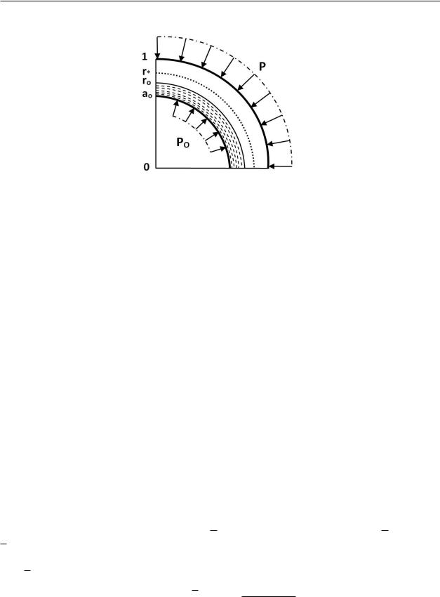
Figure 1: Design scheme for a thick-walled pipe element in an axisymmetric setting
3.2 Thick-walled element in an axisymmetric setting
First, find the axisymmetric state of the pipeline element. The axisymmetric problem for a thick-walled element is known in elasticity theory as the Lame problem. Assuming in the initial equations τrθ0 = 0, ∂σij0 /∂θ = 0, ∂K0/∂θ = 0, δ = 0 we obtain the Lame problem in the accepted formulation (Fig. 1).
The axisymmetric boundary conditions on the internal and external contour of a0 and 1 and the conjugation conditions on the contour of r0 have the form (square (round) brackets at the indices mean belonging to the plastic (elastic) zon
σ[0r] |
= P0 at r = a0; σ(0r) = P at r = 1; |
(10) |
||||
5σr0 |
6 |
= |
5σθ06 |
= 0 at r = r0 |
, |
|
|
|
|
|
|
|
|
56
Here big . . . brackets means a jump of a given value when crossing through the specifical boundary.
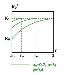
In the axisymmetric (zero) state of a thick-walled element, the softening function in the plastic zone K0 depends on the current radius r and the boundary radius r0
K0 = K (r, r0) = (K0 − K1) |
f |
(r, r0) + K1 |
(11) |
Where K0 and K1 is the value of the strength of the material on the inner contour of the element and on the elastic-plastic radius r0, f(r, r0) – some core with properties f(a0, 1) = 1, f(r0, r0) = 0. Such properties of the core allow us to describe the decrease in the value H0 not only by the radius, but also depending on the position of the boundary radius r0. As a
core f(r, r0), one can take the core [12], which well describes the softening of the material
an0 (r0n − rn) (n – nonlinearity parameter). rn(1 − an0 )
Using equilibrium equations (1), plasticity condition (3), and also axisymmetric boundary conditions and conjugation conditions (10) we find all stress components and the radius of
114 |
A.M. Alimzhanov, K.Zh. Shetiyeva |
Figure 2: Decrease in the strength parameter K0 depending on the position of the elastoplastic radius r0 according to the presented softening function K (r, r0)
the plastic zone r0.
|
r0 |
|
|
|
|
|
σ[0r] = P0 + 2a0 |
r−1K0dr, |
σ[0θ] = σ[0r] + 2K0, |
τ[0rθ] = 0 |
(12) |
||
|
|
σ(0θ) |
: = P + K1r0 1 r2 , τ(rθ) = 0 |
|
||
|
|
σ0 |
2 |
1 |
0 |
|
|
|
(r) |
|
|
||
The radius r0 is implicitly determined from the equation |
|
|||||
P0 − P + 2a0 |
r−1K0dr + K1(1 − r02) = 0 |
|
|
(13) |
||
r0 |
|
|
|
|
|
|
In the absence of corrosion damage, the parameter K0
zone r0 are found from the equation |
|
||||||
P0 |
− P + 2K1 |
ln |
a0 |
+ 2 |
$1 − r02% |
= 0 |
|
|
|
|
|
r0 |
1 |
|
|
= K1 and radius of the plastic
(14)
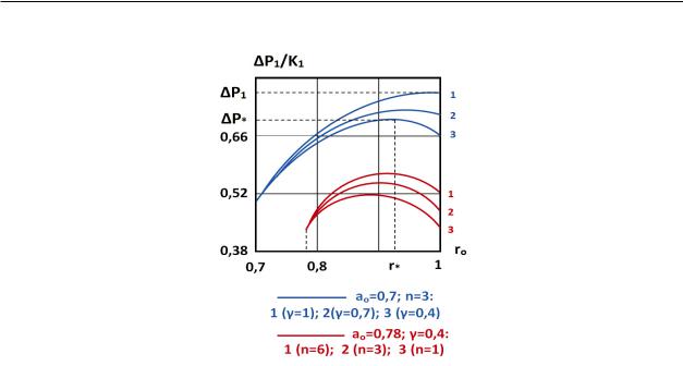
Numerical calculations were performed using formulas (11) – (14) with the following data: μ = 0, 34; E = 110GP a; P = P − P0; E = 3667K1. According to numerical results, the presence of corrosion damage a ects the elastic-plastic state of the thick-walled element. The greatest interest is the relationship P = P (r0) between value of uniform pressure P and the radius of the plastic zone r0 (Fig. 3). This dependence is determined by the thickness parameter a0 and the softening parameters of the material n, γ = K0/K1. From
Research of the stress state of an element of a thick-wall pipeline . . . |
115 |
Figure 3: The relationship between the value of uniform pressure P and the radius of the plastic zone r0 for various thickness parameters and softening parameters of the material n, γ = K0/K1
the calculations it follows that the presence of corrosion damage (γ < 1) leads to an increase in radius r0. Moreover, all curves with γ < 1 have one maximum point with an abscissa r0 = r , where a0 < r < 1. In the absence of damage (γ = 1), the radius r = 1. The existence and uniqueness of maximum points follows analytically from the nonmonotonicity and convexity of the function P = P (r0).
The maximum point characterizes the moment of loss of the bearing capacity of a thickwalled element. Corresponding to the maximum point, pressure P (ΔP ≤ P ) and radius r (r ≤ 1) are limiting for the destruction of a thick-walled element. The value r depends significantly on the thickness parameter a0 : in a thinner element, it is located closer to the inner surface (Fig. 3). The obtained results can serve as an explanation of the phenomenon of premature failure of structural elements with corrosion damage.
We denote the relationship between external loads P, P0 and radius r0 as g(P, P0, r0) = 0. Then the existence of a maximum point on the interval a0 < r0 < 1 is expressed as an additional equation ∂g(P, P0, r0)/∂r0 = 0, which has the form: K (a0, r0) − K1r02 = 0.
The bearing capacity of a thick-walled element is determined as follows. From the two transcendental equations g = 0, ∂g/∂r0 = 0, we first find the critical radius r , and then the critical loads at which the thick-walled element is destroyed.
With the known softening parameters and given external loads, it is possible to establish the optimal (minimum permissible) thickness parameter a0 for a thick-walled element of two equations g = 0, ∂g/∂r0 = 0. Calculations show that the bearing capacity of the element is significantly reduced in the presence of corrosion damage, for example, when the thickness d = 1 − a0 = 0, 4 is reduced by 12-15%. The bearing capacity of an element that allows only elastic deformation is lower by 34-50% in comparison with elastoplastic elements. It follows
116 |
A.M. Alimzhanov, K.Zh. Shetiyeva |
from the calculations that the bearing capacity of the elements increases most e ectively when their thickness increases only to d = 0.4 ÷ 0.5.
3.3Thick-walled element in a non-axisymmetric setting (outward pressure uneven in contour)
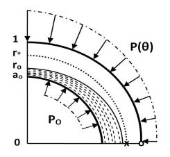
Figure 4: Design scheme for a thick-walled pipe element in a non-axisymmetric setting
Consider an extended thick-walled element loaded with an external pressure that is not uniform along the contour P (θ). The cross section of an element with an inner radius a0 and an outer radius of 1 is in plane deformation (Fig. 4).
External pressure is elliptically distributed along the contour and can be written as
P (θ) = P [1 − δ cos 2θ] |
(15) |
where P = (Pmax +Pmin)/2 is the averaged uniform pressure, δ = (Pmax −Pmin)/(Pmax +Pmin)
– a parameter characterizing the deviation of external pressure from uniform.
The solution is sought in the form (5) at ν ≥ 0. The zero solution for ν = 0 was found in the previous part of the paper. Find a solution at ν = 1. The function F (1) in (7) is represented based on the static boundary conditions (15) on the outer contour of the element:
F (1) = R(r) cos 2θ.
Solving (7), we find the function F (I) in the plastic zone: |
|
|||||||||
F (I) = |
AiRi |
+ Ri |
νi(r) dr cos 2θ, i = 1, 2, |
(16) |
||||||
|
|
r |
ν (r) |
|
|
|
|
|
|
|
|
|
a0 |
|
|
|
|||||
where AiRi |
= A1R1 + A2R2 = r(A1 cos(√ |
|
ln r) + A2 sin(√ |
|
ln r), V (r) – is the Wronskian |
|||||
3 |
3 |
|||||||||
of the solution system Ri, Vi(r) is the determinant obtained from the determinant V (r) by replacing the i-th column with a column with a single nonzero element 2K(I) cos−1 2θ located at its end.

Research of the stress state of an element of a thick-wall pipeline . . . |
117 |
Using (6), (16) we find the stress components in the plastic zone. They must satisfy the linearized boundary conditions on the inner contour
σ[(rI]) = 0, τ[(rθI)] = 0 at r = a0. |
(17) |
The components σ[(rI]), σ[(θI]), τ[(rθI)] of the stress tensor in the elastic region of the cylinder are determined from (6), (9). They satisfy the given static boundary conditions on the external contour (15) and two linearized conditions of stress conjugation σr and τγθ on the boundary
of the plastic zone: |
|
[σ[(rI])] = 0, [τ[(rθI)]] = 0 at r = r0. |
(18) |
As a result, we obtain the boundary-value problem for an elastic ring of radius r0 and 1
under the following boundary conditions: |
|
σ[(rI]) = N1(r) cos 2θ, τ[(rθI)] |
= N2(r) sin 2θ at r = r0, |
σ[(rI]) = −P cos 2θ, |
τ[(rθI)] = 0 at r = 1. |
Solving this problem, we find the stress components in the elastic region.
The equation of the boundary of the plastic zone rs is sought in the form rs = r0 + δr1. To determine the value of r1, we use the linearized conditions for the conjugation of the
components σθ and K on r0 : |
|
|
|
|
|
|
dr r1 |
9 |
|
|
|
|
|
|
|
|
|
|
|
|
|
|
|
|
|
|
|
|
|
|
|
|
|
|
|
|
|
|
|
|
|
|
|
|
|
|
||||||||||||||||||||
8σ[θ] |
+ dr r1 |
9 = 0, |
|
8K |
+ |
|
|
= 0 at |
|
r = r0, |
|
|
|
|
|
|
|
|
|
|
|
|
|
|
|
|
|
|
|
|
(19) |
|||||||||||||||||||||||||||||||||||
(I) |
|
|
|
dσθ0 |
|
|
|
|
|
|
(I) |
|
|
|
dK0 |
|
|
|
|
|
|
|
|
|
|
|
|
|
|
|
|
|
|
|
|
|
|
|
|
|
|
|
|
|
|
|
|
|
|
|
|
|
|
|
||||||||||||
where will we get it |
|
|
|
|
dr |
|
|
|
|
|
|
|
|
|
, K(I) = − dr r1 at r = r0. |
|
|
|
||||||||||||||||||||||||||||||||||||||||||||||||
|
|
|
r1 = (σθ |
− σ[θ] )/ |
− |
|
|
dr |
|
|
|
|
||||||||||||||||||||||||||||||||||||||||||||||||||||||
|
|
|
|
|
|
|
|
|
|
(I) |
(I) |
|
dσ[0θ] |
|
|
|
dσ(0θ) |
|
|
|
|
|
|
|
|
|
|
|
|
|
dK0 |
|
|
|
|
|
|
|
|
|
|
|
|
|
|
|||||||||||||||||||||
|
|
|
|
|
|
|
|
|
|
|
|
|
|
|
|
|
|
|
|
|
|
|
|
|
|
|
|
|
|
|
|
|
|
|
|
|
|
|
|
|
|
|
|
|
|
|
|
|
||||||||||||||||||
Then for r1 we will have r1 = ϕ(r0)r0 cos 2θ, where ϕ(r0) is a function of r0 : |
|
|
|
|||||||||||||||||||||||||||||||||||||||||||||||||||||||||||||||
|
|
|
|
|
|
|
ϕ(r |
) = |
|
|
|
X0 |
|
|
|
, X |
|
|
= 4(1 |
− |
r2 |
+ r−2 |
|
|
|
r4) |
−P |
, |
|
|
|
|
|
|
|
|||||||||||||||||||||||||||||||
|
|
|
|
|
|
|
|
|
|
|
|
|
|
|
|
|
|
|
|
|
|
|
|
|
|
|
|
|
|
|
||||||||||||||||||||||||||||||||||||
|
|
|
|
|
|
|
|
|
0 |
X1 + X2 + Z |
|
|
|
|
|
0 |
|
|
|
|
|
|
|
|
0 |
0 |
− 0 |
|
N |
|
|
|
|
|
|
|
|
|||||||||||||||||||||||||||||
|
|
|
|
|
|
N = 6 − 4(r02 + r0−2) + r04 + r0−4, A = |
1 |
(12 + 12α2 − α22)1/2, |
|
|
|
|||||||||||||||||||||||||||||||||||||||||||||||||||||||
|
|
|
|
|
|
|
|
|
|
|
|
|||||||||||||||||||||||||||||||||||||||||||||||||||||||
|
|
|
|
|
2 |
|
|
|
||||||||||||||||||||||||||||||||||||||||||||||||||||||||||
|
|
|
|
|
|
|
|
|
|
|
|
|
|
|
|
|
|
|
|
|
|
|
|
|
|
|
|
|
|
|
|
|
|
|
|
|
|
|
|
|
|
|
|
|
|
|
|
|
|
|
|
|
|
|
|
|
|
|
|
|
|
|
|
|
|
|
|
|
|
|
|
|
|
|
|
|
|
|
|
|
|
|
|
2 |
|
|
|
|
|
|
|
2 |
|
|
4 |
|
|
|
4 |
|
|
|
|
|
|
K |
|
|
|
|
|
|
|
|
|
|
|
|
|
|
|||||||||||||
|
|
|
|
|
|
|
|
|
|
X1 = (10 − |
4r0 |
− |
4r0− |
− r0 − r0− |
|
|
|
|
+ α1N) |
|
|
|
× |
|
|
|
|
|
|
|
|
|
|
|
|
|||||||||||||||||||||||||||||||
× ;√ |
|
|
|
|
|
|
|
|
|
|
N |
|
|
|
|
|
|
|
|
|||||||||||||||||||||||||||||||||||||||||||||||
|
cos(√ |
|
ln r0) + sin(√ |
|
ln r0) B1 + cos(√ |
|
|
|
ln r0) − |
√ |
|
sin(√ |
|
ln r0) B2 |
<, |
|
|
|||||||||||||||||||||||||||||||||||||||||||||||||
3 |
3 |
3 |
3 |
3 |
3 |
|
|
|||||||||||||||||||||||||||||||||||||||||||||||||||||||||||
|
|
|
|
|
|
|
|
|
|
|
|
|
|
|
|
|
|
|
|
|
|
|
|
|
|
|
|
|
√ |
|
|
|
|
|
|
|
|
|
|
|
|
|
|
|
|
|
|
|
√ |
|
|
|
|
|
|
|
|
|
|
|
||||||
|
|
|
|
|
|
|
|
|
|
|
2 |
|
|
4 |
|
|
|
−4 |
|
K |
|
|
|
|
|
|
|
|
|
|
|
|
|
|
|
|
|
|
|
|
|
|
|
|
|
|
|
|
|
|
||||||||||||||||
|
|
|
|
|
|
|
|
|
|
|
|
|
|
|
|
|
|
|
|
|
|
|
|
|
|
|
|
|
|
|
|
|
|
|
|
|
|
|
|
|
|
|
|
|
|
|
||||||||||||||||||||
X2 = −2(4 − 4r0 |
+ r0 − r0 |
|
) |
|
|
|
× (sin( |
3 ln r0)B1 + cos( |
|
|
|
3 ln r0)B2), |
|
|
|
|||||||||||||||||||||||||||||||||||||||||||||||||||
|
|
N |
|
|
|
|
||||||||||||||||||||||||||||||||||||||||||||||||||||||||||||
|
|
|
|
|
|
|
|
|
|
|
|
|
|
|
a0n |
|
|
|
n |
|
|
|
|
|
|
|
|
|
|
r0 |
√ |
|
|
|
|
|
|
|
π |
|
|
a0 |
|
|
√ |
|
|
|
π |
|||||||||||||||||
|
|
|
|
|
|
|
|
|
|
|
|
|
|
|
|
|
|
|
|
|
|
|
|
|
|
|
|
|
|
|
|
|
|
|
|
|
|
|
|
|||||||||||||||||||||||||||
Z = 4K1, |
|
|
K = (K0 − K1) |
|
|
|
, |
|
|
B1 = |
|
|
sin( |
|
|
|
3 ln r0 − |
|
) − |
|
|
sin( 3 ln r0 − |
|
), |
||||||||||||||||||||||||||||||||||||||||||
|
|
1 − a0n |
r0 |
|
|
2 |
|
|
3 |
2 |
3 |
|||||||||||||||||||||||||||||||||||||||||||||||||||||||
118 |
|
A.M. Alimzhanov, K.Zh. Shetiyeva |
|
|
|||||||||
|
r0 |
√ |
|
|
π |
a0 |
|
√ |
|
|
π |
||
|
|
|
|
|
|||||||||
B2 = |
|
cos( |
3 ln r0 − |
|
) − |
|
cos( |
|
3 ln r0 − |
|
) |
||
2 |
3 |
2 |
3 |
||||||||||
In the homogeneous case we have: X0 – the same thing, X1 = X2 = 0, H0 = H1, H(I) = 0
X1 = X2 = 0, K0 = K1, K(I) = 0, Z = 4K1.
Moreover, the radius r0 corresponds to the homogeneous case.
The equation of the boundary of the plastic zone rs takes the form:
rs = r0(1 + δϕ(r0) cos 2θ).
The solution exists under the condition r0(1 − δϕ(r0)) ≥ a0.
The bearing capacity of a thick-walled element can be determined from the transcendental
equation |
|
r = r0(1 + δϕ(r0)) |
(20) |
First, from (20) we find the radius r0. Substituting the found radius r0 into equation (13), we obtain critical loads at which the plastic zone reaches some "critical" points of the thick-walled element.
In the absence of corrosion damage to the element, r = 1 should be taken in equation (20) and equation (14) should be used. The critical points in this case (marked with zeros in Fig. 4) are on the external contour of the element in the directions of the minimum external pressure Pmin. In the presence of corrosion damage to the element, the critical points (marked with crosses in Fig. 4) are inside the element on circuit r in the same directions. Reaching these crosses with at least one point of the plastic zone will lead to the destruction of the element. As can be seen from Figure 4, the plastic zone is elongated in the directions of action of Pmin. Damage to the material leads to an increase in the size of the plastic zone. The degree of damage to the material depends on the size of this zone. The element has the greatest damage in the directions of action of Pmin. Therefore, the softening of the element depends both on the size of the plastic zone and on the orientation of its boundary.
4 Conclusion
The stress-strain state of an elastoplastic element of a thick-walled pipeline is studied under conditions of force and corrosion using a special softening function (plastic inhomogeneity) in the plasticity condition of Tresca-Saint-Venant.
The elastoplastic problem for a thick-walled element in an axisymmetric formulation (with uniform external and internal pressure) and non-axisymmetric formulation (with an external pressure uneven in contour) is considered. The problems are solved by the method of sharing static and physical equations and the perturbation method in the theory of an elastoplastic body.
An assessment of the strength and bearing capacity of a thick-walled element under corrosive force is given.

Research of the stress state of an element of a thick-wall pipeline . . . |
119 |
References
[1]СНиП 3.05-01-2010. "Magistral’nye truboprovody [Trunk pipelines]".
[2]СП 33.13330.2012. "Raschet na prochnost’ stal’nyh truboprovodov [Strength analysis of steel pipelines]".
[3]Gareev A.G., Nasibullina O.A. and Rizvanov R.G., "Izuchenie korrozionnogo rastreskivaniya magistral’nyh gazonefteprovodov [The study of corrosion cracking of gas and oil pipelines]" , Oil and gas business 6 (2012), http://www.ogbus.ru/ authors/Gareev2.pdf.
[4]Basiyev K.D. et al., "Issledovanie processov zarozhdeniya i razvitiya korrozionno-mekhanicheskih treshchin na poverhnosti trub [Study of the processes of nucleation and development of corrosion-mechanical cracks on the surface of pipes]" ,
Bulletin of the Vladikavkaz Scientific Center 3 (2014): 56-61.
[5]Cherepanov G.P., Mekhanika hrupkogo razrusheniya [Mechanics of brittle fracture] (Moscow: Science, 1974): 640.
[6]Astafiev V.I., Radayev U.N. and Stepanova L.V., Nelinejnaya mekhanika razrusheniya [Nonlinear fracture mechanics] (Samara: SamSU Publishing House, 2001): 562.
[7]Sadyrin A.I., "Modeli nakopleniya povrezhdenij i kriterii razrusheniya konstrukcionnyh uprugoplasticheskih materialov pri dinamicheskom nagruzhenii [Damage accumulation models and fracture criteria of structural elastoplastic materials under dynamic loading]" , Problems of strength and plasticity 74 (2012): 28-39.
[8]Rossina N.G. et al., Korroziya i zashchita metallov. CHast’1. Metody issledovanij korrozionnyh processov [Corrosion and metal protection. Part 1. Research methods for corrosion processes] (Ekaterinburg: Ural University Publishing House, 2019): 108.
[9]Kushrin S.Ya., Mosyagin M.N. and Pesin A.S., Processy razvitiya korrozionnyh treshchin pod napryazheniem magistral’nyh gazoprovodov pod vliyaniem izmeneniya ih vysotnogo polozheniya i katodnoj zashchity [Processes of development of corrosion cracks under stress of main gas pipelines under the influence of changes in their altitude position and cathodic protection] (St.Petersburg: Nedra, 2010): 168.
[10]Ovchinnikov I.I., "Issledovanie povedeniya obolochechnyh konstrukcij, ekspluatiruyushchihsya v sredah, vyzyvayushchih korrozionnoe rastreskivanie [Study of the behavior of shell structures operating in environments that cause corrosion cracking]" , Science 4 (2012): 1-30.
[11]Alimzhanov M.T., "Uprugoplasticheskaya zadacha, uchityvayushchaya neodnorodnost’ mekhanicheskih svojstv materiala [Elastic-plastic problem, taking into account the heterogeneity of the mechanical properties of the material]" , Reports of the USSR Academy of Sciences 6 (1978): 1281-1284.
[12]Alimzhanov M.T., "O nakoplenii povrezhdenij i nesushchej sposobnosti elementov tolstostennyh konstrukcij [On the accumulation of damage and bearing capacity of elements of thick-walled structures]" , International journal Problems of mechanical engineering and automation 1 (1992): 58-64.
[13]Alimzhanov A.M., "Dvumernaya uprugoplasticheskaya zadacha s lokal’noj plasticheskoj neodnorodnost’yu [Twodimensional elastic-plastic problem from the local plastic inhomogeneity]" , Mechanics and modeling of technology processes 1 (1997): 3-17.
[14]Alimzhanov A.M., "Ploskaya uprugoplasticheskaya zadacha dlya neodnorodnogo tela s otverstiem [Flat elastic-plastic problem for a non-uniform body with a hole]" , Bulletin of the Russian Academy of Sciences. Mechanics of solids 2 (1998): 119-138.
[15]Ivlev D.D. and Ershov L.V., Metod vozmushchenij v teorii uprugoplasticheskogo tela [The perturbation method in the theory of an elastoplastic body] (Moscow: Science, 1978).
120ISSN 1563-0277, eISSN 2617-4871 |
Journal of Mathematics, Mechanics, Computer Science. № 1(105). 2020 |
IRSTI 27.35.25 |
https://doi.org/10.26577/JMMCS.2020.v105.i1.11 |
1N.T. Azhikhanov, 2B.T. Zhumagulov, 3T.A. Turymbetov, 4A.B. Bekbolatov
1Doctor of Technical Sciences, Academy of Public Administration under the President of Kazakhstan, Turkestan, Kazakhstan, E-mail: ajihanov1@mail.ru
2Doctor of Technical Sciences, Academician of NAS RK, National Engineering Academy of the Republic of Kazakhstan, Almaty, Kazakhstan, E-mail: zhumagulov_b@mail.ru
3Candidate of Technical Sciences, Khoja Akhmet Yassawi International Kazakh-Turkish University, Turkestan, Kazakhstan, E-mail: tursinbay@mail.ru
4PhD student, Khoja Akhmet Yassawi International Kazakh-Turkish University, Turkestan, Kazakhstan, E-mail: alimzhan_iktu@mail.ru
STRESSED-DEFORMED STATE OF TWO DRIFTS IN A TILTLY LAYERED CRACKED ARRAY IN THE CONDITIONS OF ELASTIC DEFORMATIONS OF ROCKS
In the study, based on a homogeneous anisotropic mechanical-mathematical model of an inclined, finely layered array with a biperiodic system of slots, the patterns of distribution of elastic stresses and displacements near two drifts of arbitrary profile shape and depth by the finite element method under conditions of plane deformation have been systematically numerically investigated. The calculation was carried out by converting weakened rocks with two excavations in elasticity to an equivalent homogeneous medium. It is di cult to solve the problem of the initial static stress state of two-diagonal workings on a rock weakened by two-period cracks by the analogous method, therefore it was solved by the generalized method of plane deformation using the first and second isoparametric elements by the finite element method. Methods for dividing the area specified by the finite element method into parametric quadrangular elements and numerically determining the stress-strain state of double workings are given.
A computational algorithm has been developed and a software package has been developed for studying the elastic state of adjacent cavities of arbitrary depth and shape. A multivariate numerical calculation and analysis of the influence on the components of stresses and displacements near cavities, geometrical, physical parameters of rocks was carried out.
Key words: drift, isoparametric element, transtropic array, finite element method.
1Н.Т. Ажиханов, 2Б.Т. Жұмағұлов, 3Т.А. Тұрымбетов, 4А.Б. Бекболатов
1т.ғ.д., Қазақстан Республикасы Президентiнiң жанындағы мемлекеттiк басқару академиясы, Түркiстан қ., Қазақстан, E-mail: ajihanov1@mail.ru
2т.ғ.д., ҚР ҰҒА академигi, Қазақстан Республикасының ұлттық инженерлiк академиясы, Алматы қ., Қазақстан, E-mail: zhumagulov_b@mail.ru
3т.ғ.к., Қожа Ахмет Ясауи атындағы Халықаралық қазақ-түрiк университетi, Түркiстан қ., Қазақстан, E-mail: tursinbay@mail.ru
4PhD докторант, Қожа Ахмет Ясауи атындағы Халықаралық қазақ-түрiк университетi, Түркiстан қ., Қазақстан, E-mail: alimzhan_iktu@mail.ru
Екi штректiң серпiмдi тау жыныстарынының жарықтары массивтi салмақты қабаттағы кернеулiк-деформациялық жағдайы
Зерттеуде бипериодты саңылаулар жүйесi бар көлбеу, жұқа қабатты массивтiк бiртектi анизотропты механикалық-математикалық моделiн ала отырып, жазықтықтың деформациялану жағдайына шектi элемент әдiсiн қолдандық және тереңдiктiң екi штректiң маңайында серпiмдi кернеулер мен орын ауыстырулардың заңдылықтары жүйелi түрде зерттелдi. Тау жыныстарының геометриялық, физикалық параметрлерiне кернеулер мен орын ауыстырулар компоненттерiне әсер етудi сандық есептеу және талдау жүргiзiлдi.
c 2020 Al-Farabi Kazakh National University