

83
.pdfV.Folomeev et al.
В.Фоломеев1,2*, Б. Клейхаус3, Ж. Кунц3
1Институт физики им. академика Ж. Жеэнбаева НАН Кыргызской Республики, Кыргызстан, г. Бишкек, 2Международная лаборатория теоретической космологии, Томский государственный университет систем управления и радиоэлектроники (ТУСУР), Россия, г. Томск
3Институт физики, Олденбургский университет, Германия, г. Олденбург, *е-mail: vfolomeev@mail.ru
Смешанные системы звезда плюс кротовая нора с комплексным скалярным полем
Мы исследуем компактные смешанные конфигурации с нетривиальной топологией пространства-времени типа кротовой норы, образованные комплексным скалярным полем с четверичной потенциальной энергией и политропной жидкостью. Последняя моделируется релятивистским баротропным уравнением состояния, которое может приближенно описывать более или менее реалистичное вещество. Для таких систем мы находим регулярные асимптотически плоские равновесные решения, описывающие локализованные конфигурации, в которых жидкость сконцентрирована в области с конечными размерами. Полученные решения описывают кротовые норы с двумя горловинами, которые расположены вне жидкости (можно сказать, что жидкость скрыта в области между горловинами). Также мы рассматриваем зависимость полной массы системы от центральной плотности жидкости и демонстрируем существование критических значений центральной плотности, при которых масса расходится. При этом все регулярные решения с конечными массами лежат в области между критическими значениями, и эта область также содержит разрыв в значениях центральной плотности, в котором имеются только физически неприемлемые осциллирующие решения. Показано, что для некоторых значений центральной плотности жидкости могут существовать решения, описывающие системы, в которых максимумы плотности жидкости и ее давления лежат не в центре конфигурации. Это приводит к тому, что такие системы обладают двумя экваторами (локальными максимумами метрической функции), расположенными симметрично относительно центра.
Ключевые слова: кротовые норы, нетривиальная топология, комплексные скалярные поля, политропная жидкость.
Introduction
At the present time various scalar fields play an important role in constructing models of the early and present Universe. In particular, they may provide both the inflationary stage in the very early Universe and its current accelerated expansion [1]. Theirroleonsmallspatialscalescomparabletosizes of galaxies and their clusters, as well as on scales of stars, can also be significant. Namely, one can imagine a configuration consisting of a scalar field confined by its own gravitational field – a boson star [2, 3]. Due to the quantum Heisenberg uncertainty principle, there is a pressure inside such a star preventing it from gravitational collapse. In this sensesuchascalarstarisasortofquantum-classical objectwhoseexistenceisensuredsimultaneouslyby quantum and classical properties of the scalar field. The studies performed in the literature indicate that masses of such objects can vary from atomic ones (“gravitational atom”) to masses of the order of the Chandrasekhar mass, and even much larger. It is not impossiblethattherecanbemanysuchobjectsinthe Universe. Then, if their electromagnetic radiation is
weak,theycanserveascandidatesfortheroleofthe missing dark matter.
In constructing models of boson stars, two types of scalar fields are used – real and complex ones [2, 3].Indoingso,usuallyacanonicalfieldisemployed with a fixed sign in front of the kinetic term of the scalar field Lagrangian density. If one takes the other sign, this corresponds to so-called ghost scalar fields. The possible existence of such fields in nature is indirectly supported by the observed accelerated expansion of the present Universe (see, e.g., Ref. [4]). As the canonical scalar fields, ghost fields enable one to get localized static nonsingular solutions both with a trivial spacetime topology [5] and with a nontrivial one – the so-called wormholes [6-10]. If ordinary matter or radiation can fill such wormholes, they are called traversable wormholes (for a generaloverviewon the subject,seethebooks [11, 12]). As matter threading the wormhole, one can use, for example, a relativistic fluid of the type containinginneutronstars.Thenthemixedneutron- star-plus-wormhole configurations will possess properties of wormholes and of ordinary stars [1319].
11

Mixed star-plus-wormhole systems with a complex scalar field
The goal of the present paper is to study a wormholesupported by acomplex ghost scalarfield and filled with ordinary matter. To do this, we will construct localized regular solutions with a nontrivial wormholelike topology. In two limiting cases, such a system becomes the system consisting of a wormhole only (without ordinary matter) [20] or the mixed system supported by a massless real scalar field [16]. Our purpose will be to find out
what are the differences between the configurations considered here and the systems of Refs. [16, 20].
General equations
We consider a model of a mixed gravitating configuration consisting of a complex ghost scalar field and polytropic fluid. The corresponding action for such a system can be taken in the form
(|Φ| |
) |
|
|
|
fl |
|
= ∫ 4 − −163 |
|
+ 21 − ∂ Φ |
∂ Φ |
− (|Φ|2) + fl, |
|
|
|
|
|
|
|
|
(1) |
||||||||||||||||||||||||||||||||||
|
|
|
|
|
isacomplex scalar field with the potential |
|
|
Our goal here is to study equilibrium |
||||||||||||||||||||||||||||||||||||||||||||||
where Φ and |
|
denotes |
the |
action of |
|
the |
fluid. |
wormhole-plus-fluid solutions. To this end, it is |
||||||||||||||||||||||||||||||||||||||||||||||
0,1,2,3 |
. |
|
|
|
|
|
|
|
|
|
|
|
|
|
|
|
|
|
, . . . = |
in polar Gaussian coordinates |
|
|
|
|
|
|
|
|
|
|
|
|||||||||||||||||||||||
Hereafter2 |
|
the Greek indices run over |
|
|
|
|
|
convenient to take the spherically symmetric metric |
||||||||||||||||||||||||||||||||||||||||||||||
right-hand side contains the energy-momentum |
|
2 |
= |
|
( |
0 |
) |
2 |
− |
|
2 |
− |
2 |
(Θ |
2 |
+ sin Θ |
2 |
), |
||||||||||||||||||||||||||||||||||||
can |
|
obtain |
the |
gravitational |
equations |
whose |
|
|
|
|
|
|
|
|
|
|
|
|
|
|
|
|
2 |
|
|
|
||||||||||||||||||||||||||||
|
By varying (1) with respect to the metric, one |
|
|
|
|
|
|
|
|
|
|
|
|
|
|
|
|
|
|
|
|
|
|
|
|
|
|
|
||||||||||||||||||||||||||
|
|
|
|
|
|
|
|
|
|
|
|
|
|
|
|
|
|
|
|
|
|
|
|
|
|
|
|
|
|
|
|
|
|
|
|
|
|
|
|
|
|
|
|
|
|
with |
|
a |
||||||
tensor |
|
|
|
|
|
|
|
|
|
|
|
|
|
|
|
|
|
|
|
|
|
|
|
|
|
We |
will |
|
study localized solutions |
|
||||||||||||||||||||||||
|
|
|
= −2 (∂ Φ ∂ Φ + ∂ Φ∂ Φ ) + |
|
where |
|
|
and |
|
|
|
|
are |
functions |
of |
the |
radial |
|||||||||||||||||||||||||||||||||||||
|
|
|
|
|
|
presence of the complex ghost scalar field in the |
||||||||||||||||||||||||||||||||||||||||||||||||
|
|
|
|
|
|
|||||||||||||||||||||||||||||||||||||||||||||||||
|
|
|
|
|
|
|
1 |
|
|
|
|
|
|
|
|
|
|
|
|
|
|
|
|
|
coordinate |
|
only. |
|
|
|
|
|
|
|
|
|
|
|
|
|
|
|
|
|||||||||||
|
|
|
|
|
|
|
|
∂ Φ |
|
∂ Φ |
+ + |
|
|
|
|
|
wormholelike topology, which is ensured by the |
|||||||||||||||||||||||||||||||||||||
|
|
|
|
|
+ 2 |
|
|
|
|
|
|
|
|
|
for the scalar field the harmonic ansatz |
|
|
|
|
|
|
|||||||||||||||||||||||||||||||||
|
|
|
|
|
|
1 |
|
|
|
|
|
|
|
|
|
|
|
|
|
|
|
|
|
dependence in the gravitational equations, we use |
||||||||||||||||||||||||||||||
|
|
|
|
|
|
|
+( |
+ ) − , |
|
|
|
|
|
|
|
action |
(1). |
|
Then, |
in |
|
order |
|
to |
|
have no |
time |
|||||||||||||||||||||||||||
|
|
|
|
|
|
|
|
|
|
|
|
|
|
|
|
|
|
|
|
|
|
Φ( |
|
, ) = ( ) |
|
|
|
, |
|
|
|
|
|
|
||||||||||||||||||||
its pressure. In turn, varying (1) with respect to the |
which |
|
|
|
|
|
|
|
|
|
of |
|
|
the |
||||||||||||||||||||||||||||||||||||||||
where |
|
is the energy density of the fluid and |
|
is |
ensures |
|
0 |
that |
|
the |
|
spacetime |
|
|
||||||||||||||||||||||||||||||||||||||||
|
|
|
|
|
|
|
|
|
|
|
|
|
|
|
|
|
|
|
|
−0 |
|
|
|
|
|
|
|
|||||||||||||||||||||||||||
scalar field, one obtains the equation for |
|
|
, |
|
|
|
|
equations: |
|
|
|
|
|
|
|
|
|
|
|
|
|
|
|
|
|
|
|
|
|
|
|
|||||||||||||||||||||||
|
|
|
1 |
|
∂ |
|
|
|
|
|
|
|
∂Φ |
|
|
|
|
|
|
|
|
|
|
|
|
|
|
|
|
|
|
|
|
|
|
|
|
|
|
|
|
|
|
|
||||||||||
|
|
− |
∂ − |
|
∂ = |Φ|2 |
Φ.\ |
|
|
|
configurationunderconsideration remainsstatic.As |
||||||||||||||||||||||||||||||||||||||||||||
|
|
|
|
|
|
|
|
|
|
|
|
|
|
|
|
|
|
|
Φ |
|
|
|
|
|
a result, we have the following set of Einstein-scalar |
|||||||||||||||||||||||||||||
|
|
|
|
|
|
− 2 ′′ + ′ 2 |
+ 12 = 8 4 00 |
= 8 4 + |
21 [−( ′2 + 2 − 2) + ] , |
|
|
|
|
|
|
|
|
(2) |
||||||||||||||||||||||||||||||||||||
|
|
|
′′ + 21 |
− |
′ |
′ |
+ ′ + 12 = 8 4 |
11 = 8 4 |
− + 21 ( ′2 |
+ 2 |
− |
|
2 + ) , |
|
+ ] , |
|
|
|
|
|
(3) |
|||||||||||||||||||||||||||||||||
|
|
|
′ ′ |
+ 21 |
′′ |
+ 41 |
′2 |
= −8 4 |
22 |
= − |
8 4 − |
+ 21 [−( ′2 |
− |
2 − 2) |
|
|
|
|
|
(4) |
||||||||||||||||||||||||||||||||||
|
|
|
|
|
|
|
|
|
|
|
|
|
′′ |
+ 21 ′ + 2 ′ ′ |
+ 2 − |
+ |Φ|2 |
= 0, |
|
|
|
|
|
|
|
|
|
|
|
|
(5) |
||||||||||||||||||||||||
|
|
|
|
|
|
|
|
|
|
|
|
|
|
|
|
|
|
|
|
|
|
|
|
|
and the boundary conditions, it is possible to |
|||||||||||||||||||||||||||||
where the prime denotes differentiation with respect |
|
|||||||||||||||||||||||||||||||||||||||||||||||||||||
to |
|
. Depending on the specific form of the potential |
obtain |
localized |
equilibrium |
|
solutions |
by |
solving |
|||||||||||||||||||||||||||||||||||||||||||||
12

V. Folomeev et al.
these equations numerically. Notice here that in the |
||
of |
In order to obtain=regular= 0 asymptotically flat |
|
absence of the fluid we return to the system of Ref. |
||
[20]. In turn, when |
, we have the system |
|
|
Ref. [16]. |
|
solutions with a nontrivial topology, we take the
potential |
= − 2 |
|
|Φ|2 + 21 |Φ|4, |
|
||
|
|
|
||||
Next, |
|
|
2 |
2 |
|
(6) |
|
|
|||||
the |
above equations have |
to be |
||||
where |
and |
|
are free parameters of the scalar |
|||
field. |
|
̅ |
|
|
|
|
supplemented by an equation of state for the fluid.
We consider here the simplest case of a barotropic equation of state where the pressure is a function of the mass density . Namely, we take the following
polytropic equation of state that can approximately
describe more or less realistic matter:
|
|
|
|
= 1+1/ , |
= 2 + , |
|
|
|
|
(7) |
|||||||||||||||
polytropic |
index |
|
|
|
= |
2 |
( , |
|
) |
|
|
|
|
|
|||||||||||
where |
the |
constant |
|
|
|
|
|
|
|
( ) |
|
1− |
, |
the |
|||||||||||
denotes the rest- |
|
|
= 1/( − 1) |
|
and |
|
= |
|
|||||||||||||||||
is |
the baryon |
|
number |
density, |
|
( ) |
|
is a |
|||||||||||||||||
|
|
|
|
|
|
|
|
|
|
|
|
, |
|
|
|
is the |
|
|
|
|
|
|
|||
|
|
|
|
|
|
mass density of the fluid. Here |
|
|
|||||||||||||||||
on the properties of the |
|
matter. |
For the sake of |
||||||||||||||||||||||
simplicity, |
we |
take here only one set of parameters |
|||||||||||||||||||||||
characteristic value of |
|
|
|
|
|
|
|
|
|
baryon mass, |
|||||||||||||||
and |
|
and |
are parameters whose values depend |
||||||||||||||||||||||
|
= 1.66 × 10 |
−24 |
g |
|
|
|
= 0.1 fm |
|
= 0.1 |
|
|||||||||||||||
|
|
= 2 |
|
|
|
, |
|
( ) |
|
|
|
|
|
−3, |
|
|
|
|
, |
||||||
and |
[21], and employ them in the numerical |
||||||||||||||||||||||||
|
Then, introducing the new variable |
, |
|
|
|
|
|
||||||||||||||||||
calculations of Sec. 3. |
|
|
|
|
|
|
|
|
|
|
|
|
|
|
|
|
|
||||||||
where |
|
is the central=density, |
of the fluid, we can |
||||||||||||||||||||||
(7) as |
|
|
|
|
|
|
|
|
|
|
|
|
|
|
|
|
|
|
|
|
|
|
|
||
rewrite the pressure and the energy density from Eq. |
|||||||||||||||||||||||||
= |
|
|
+1, |
= 2 |
+ |
|
|
. |
|
||||||||||||||||
|
|
1+1/ |
|
|
|
|
|
|
|
|
|
|
|
|
|
|
1+1/ |
|
|
|
|
||||
|
Making use of these expressions and of the |
||||||||||||||||
equation that follows from the |
|
|
|
|
component of |
||||||||||||
the law of conservation of |
energy and momentum, |
||||||||||||||||
|
= |
|
|
||||||||||||||
|
|
, |
|
= −1 ( + ) , |
|
|
|
||||||||||
; = 0 |
|
|
|
|
|
||||||||||||
|
|
|
|
|
internal region with |
|
, |
|
|||||||||
we have for the |
|
|
|
|
2 |
|
|
|
≠ 0 |
|
|||||||
|
2 ( + 1) |
|
|
= −[1 + ( + 1) ] , |
(8) |
||||||||||||
where |
|
|
1/ |
|
|
|
|
|
related2 |
is a |
dimen- |
||||||
|
|
relativity parameter,2 |
to the central |
||||||||||||||
sionless = |
|
/ |
|
= /( |
) |
|
|
|
|||||||||
pressure |
of the fluid. Integrating this equation, |
||||||||||||||||
we get the metric function |
|
in terms of |
, |
||||||||||||||
|
|
|
|
= |
|
|
1 + ( + 1) |
2 |
|
||||||||
and. The |
|
|
|
1 + ( + 1) , |
|
||||||||||||
is the value of |
|
at the center where |
|||||||||||||||
integration |
|
constant |
|
|
|
|
|
the |
|||||||||
|
|
|
of |
the |
|
|
|
|
|
|
is |
|
fixed |
by = |
|||
requirement |
|
asymptotic |
flatness |
of the |
|||||||||||||
1 |
|
|
|
|
|
|
→ |
|
|
|
|
|
|
|
|
|
|
spacetime, i.e., |
|
1 at infinity. |
|
|
|
|
|||||||||||
Numerical solutions
Let us now turn to the numerical calculations. For this purpose, it is convenient to rewrite the above equations in terms of the dimensionless
variables |
= |
|
, = |
, Ω = , Λ = |
|
|||||||||
|
|
|
|
|
|
|
|
|
|
√4 |
|
(9) |
||
|
|
|
|
|
|
2 |
|
̅ |
|
|||||
|
|
= 4 |
|
|
|
2 |
, |
|
||||||
|
|
|
|
, = |
|
|
|
|||||||
where |
= / |
is |
the |
constant having |
the |
|||||||||
length). |
Then, |
using the potential (6), one can |
||||||||||||
dimensions of length (since we consider a classical |
||||||||||||||
theory, |
|
neednotbeassociatedwiththeCompton |
||||||||||||
rewrite Eqs. (2)-(5) in the form
− 2 ′′ |
+ ′ 2 + 12 |
= (1 + ) − ′2 − Ω2 − 2 |
− 2 |
+ Λ2 |
4, |
(10) |
|
− ′ ′ + ′ + 12 = −+1 + ′2 + Ω2 − 2 − |
2 + |
Λ2 4 |
, |
, |
(11) |
||
′′ + 21 |
′ ′ + 21 ′′ + |
41 ′2 = +1 + ′2 − Ω2 − 2 + 2 − Λ2 4 |
(12) |
||||
13

Mixed star-plus-wormhole systems with a complex scalar field
one may |
|
|
|
|
|
|
|
|
|
|
|
|
|
|
|
|
|
|
|
′′ + 21 |
′ |
+ 2 ′ |
′ + (Ω2 − − 1 + Λ2) |
= 0, |
|
|
|
|
|
|
|
|
|
|
|
|
(13) |
|||||||||||||||||||||||||||||||||||
use= 8any three/of |
themin calculations. Here, |
configurations2 |
under consideration. |
|
|
|
|
|
|
|
|
|||||||||||||||||||||||||||||||||||||||||||||||||||||||||||||
where |
|
|
|
|
|
|
|
|
|
|
|
|
|
|
|
|
|
|
|
|
|
|
|
|
|
. Since, due to the Bianchi |
constant |
|
|
|
|
|
plays the role of the Arnowitt-Deser- |
|||||||||||||||||||||||||||||||||||||||
identities,notallof2 these2equationsareindependent, |
Misner (ADM) mass of the wormhole-plus-fluid |
|||||||||||||||||||||||||||||||||||||||||||||||||||||||||||||||||||||||
we will solve Eqs. (8), (10), (12), and (13), treating |
We solve the set of equations (8) and (10)-(13) |
|||||||||||||||||||||||||||||||||||||||||||||||||||||||||||||||||||||||
the first-order equation (11) as a constraint equation |
numerically,usingtheboundary conditions(14) and |
|||||||||||||||||||||||||||||||||||||||||||||||||||||||||||||||||||||||
to check the accuracy of the computations. |
|
|
|
|
|
|
(15)andvaryingthevalueofthebosonfrequency |
Ω |
||||||||||||||||||||||||||||||||||||||||||||||||||||||||||||||||
When solving the above equations, we use the |
in the interval |
|
|
|
|
|
|
|
|
|
[the lower limit |
|
|
|
||||||||||||||||||||||||||||||||||||||||||||||||||||||||||
symmetric |
|
boundary |
|
conditions |
imposed |
at |
|
the |
|
|
|
|
|
|
|
|
|
|
|
|
||||||||||||||||||||||||||||||||||||||||||||||||||||
|
|
|
|
|
|
|
|
|
|
|
|
|
|
|
|
|
|
|
|
|
|
|
|
|
|
|
|
|
|
|
|
|
|
|
|
|
|
|
|
|
|
|
|
|
corresponds to |
the case of real scalar fields and the |
||||||||||||||||||||||||||
center |
|
|
|
|
|
|
|
|
, |
|
|
|
|
|
|
|
|
|
|
|
|
|
|
|
|
|
|
|
|
|
|
|
|
|
|
|
|
|
|
|
|
|
0 ≤ Ω ≤ 1 |
|
|
|
|
|
|
|
Ω = 0 |
|||||||||||||||||||||
|
|
|
|
(0) = |
, (0) = , (0) = , (0) = 1 |
consideration may be subdivided into two regions: |
||||||||||||||||||||||||||||||||||||||||||||||||||||||||||||||||||
|
|
|
|
|
= 0 |
|
|
|
|
|
|
|
|
|
|
|
|
|
|
|
|
|
|
|
|
|
|
|
|
|
|
|
|
|
|
|
|
|
|
nonoscillating asymptotic behavior of the scalar |
||||||||||||||||||||||||||||||||
|
|
|
|
|
|
|
|
|
|
|
|
|
|
|
|
|
|
|
|
|
|
|
|
|
|
|
|
|
|
|
|
|
|
|
|
|
|
|
|
|
|
(14) |
field; see Eq. (17)]. In doing so, the systems under |
|||||||||||||||||||||||||||||
|
|
|
|
|
|
|
|
|
|
|
|
|
|
|
|
|
|
|
|
|
|
|
|
|
|
|
|
|
|
|
|
|
|
|
|
|
|
|
|
|
|
(i) the internal one, where both the fluid and the |
||||||||||||||||||||||||||||||
(all first-order derivatives are supposed to be zero at |
||||||||||||||||||||||||||||||||||||||||||||||||||||||||||||||||||||||||
scalar field are present; (ii) the external one, where |
||||||||||||||||||||||||||||||||||||||||||||||||||||||||||||||||||||||||
the center). The constraint equation (11) then yields |
only the scalar field is present. Correspondingly, the |
|||||||||||||||||||||||||||||||||||||||||||||||||||||||||||||||||||||||
|
|
|
= |
Ω |
|
|
|
|
|
|
|
−1+(Λ/2) |
−. |
|
|
|
|
|
|
|
|
|
the external ones at the edge of the fluid, |
|
|
|
|
|
. |
|||||||||||||||||||||||||||||||||||||||||||
|
|
|
|
|
|
|
|
|
|
2 |
|
|
|
2 |
|
− |
|
|
|
|
|
|
2 |
|
|
|
|
|
|
|
|
|
|
|
|
|
|
solutionsintheexternalregioncanbeobtainedfrom |
||||||||||||||||||||||||||||||||||
|
|
|
|
|
|
|
|
|
|
|
|
|
|
1 |
|
|
|
|
|
|
|
|
|
|
|
|
|
|
|
|
|
zero. The internal solutions should be matched with |
||||||||||||||||||||||||||||||||||||||||
|
|
|
|
|
|
|
|
|
|
|
|
|
|
|
|
|
|
|
|
|
|
|
|
|
|
|
|
|
|
|
|
|
|
|
|
|
|
|
|
(15) |
Eqs. (10)-(13), where the function |
is set to be |
||||||||||||||||||||||||||||||
Using |
|
this |
|
|
|
|
expression |
and |
expanding |
|
|
the |
This is done by equating the corresponding |
= |
|
|||||||||||||||||||||||||||||||||||||||||||||||||||||||||
|
|
|
|
|
|
|
|
|
|
|
2 |
|
, |
|
|
|
one |
can find |
|
from |
Eq. |
(10) |
|
the |
boundary ofthe |
|
|
|
|
|
|
|
|
|
|
|
|
|
|
|
|
can |
||||||||||||||||||||||||||||||
|
|
|
|
|
|
|
|
|
|
|
|
|
|
|
|
|
|
|
|
|
|
|
|
|
|
|
|
|
|
|
|
|
|
|
|
|
|
|
≈ |
|
|
|
. In turn, the integration constant |
|
|
|
||||||||||||||||||||||||||
value |
of the2second derivative of |
|
|
|
|
|
|
|
|
|
|
|
|
|
|
|
|
|
|
|
|
|
|
|
|
|
|
|
|
|
|
|
|
|
|
|
values |
|||||||||||||||||||||||||||||||||||
|
|
at the center |
|
|
|
|
|
|
|
|
|
|
|
|
|
|
|
|
|
|
|
|
|
|
|
|
|
|
|
|||||||||||||||||||||||||||||||||||||||||||
+ 1/2 |
|
|
|
the |
|
vicinity |
of |
|
the |
center |
as |
|
|
|
|
be determined from the |
and their derivatives. The |
|||||||||||||||||||||||||||||||||||||||||||||||||||||||
function |
|
|
|
in |
|
|
|
|
|
|
|
of the functions |
|
|
, |
|
, |
|
||||||||||||||||||||||||||||||||||||||||||||||||||||||
|
|
|
|
|
|
|
|
|
|
|
|
|
|
|
|
|
|
|
|
|
|
|
|
|
|
|
|
|
|
|
|
|
|
|
|
|
|
|
|
|
|
|
|
( ) = 0 |
|
|
|
solutions, proceeding |
|
|
|
the |
||||||||||||||||||||
|
|
|
|
|
|
|
|
|
|
|
|
|
|
|
|
|
|
|
|
|
|
|
|
|
|
|
|
|
|
|
|
|
|
|
|
|
|
|
|
|
|
|
asymptotic |
|
|
from |
||||||||||||||||||||||||||
2 |
= 2 {2Ω |
|
|
|
|
|
|
|
|
|
− [1 + ( |
+ 1)]}. |
|
|
|
|
|
|
|
|
|
|
|
|
|
fluid |
|
|
is defined by thecondition |
|||||||||||||||||||||||||||||||||||||||||||
2 |
− |
|
|
|
|
|
asymptotically flat. |
|
|
|
|
|
|
|
|
|
|
|
|
|
|
|
|
|||||||||||||||||||||||||||||||||||||||||||||||||
|
|
|
|
|
|
|
|
|
|
|
|
|
|
|
|
2 |
|
|
|
|
|
|
|
|
|
|
|
|
|
|
|
|
|
(16) |
requirement that the external solutions must be |
|||||||||||||||||||||||||||||||||||||
asinthecaseofbosonstars[22],assuch |
|
aparameter,Ω |
typical solutions for the scalar field function |
|
|
, the |
||||||||||||||||||||||||||||||||||||||||||||||||||||||||||||||||||
one |
can |
take |
|
|
|
|
|
|
. Then, |
the other |
|
two |
|
parameters |
fluid function |
|
|
, and the metric function |
|
|
. The |
|||||||||||||||||||||||||||||||||||||||||||||||||||
Thus we have threeparameters – |
|
|
, |
|
, and |
|
, |
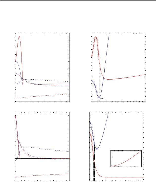
In the left panels of figure 1, we show a set of |
||||||||||||||||||||||||||||||||||||||||||||||||||||||||||||||||
should |
|
|
be |
|
chosen in such a way as to ensure |
value of the |
|
|
|
|
|
|
|
|
|
|
|
|
|
|
|
|
|
|
||||||||||||||||||||||||||||||||||||||||||||||||
one of which can be chosen arbitrarily. For instance, |
|
|
|
|
|
|
|
|
|
|
|
|
|
|
|
|
|
|
|
|
|
|
|
|
|
|
|
|||||||||||||||||||||||||||||||||||||||||||||
and |
|
|
|
|
|
|
|
|
|
|
|
|
|
|
|
|
|
|
|
|
. In this sense, we |
|
|
|
|
|
|
limiting value of the physically acceptable interval. |
||||||||||||||||||||||||||||||||||||||||||||
|
|
|
|
|
|
|
|
and |
|
|
|
|
|
|
|
|
|
|
|
|
|
|
|
limiting |
|
case |
|
|
|
|
|
|
is |
|
|
undistinguishable |
|
since |
||||||||||||||||||||||||||||||||||
|
|
|
|
|
|
|
|
|
|
|
|
|
|
|
|
|
|
|
|
|
|
|
|
|
|
|
|
|
|
|
|
|
|
|
|
|
|
|
|
|
|
|
|
|
|
|
|
|
|
|
boson frequency |
|
|
represents the |
||||||||||||||||||
with an eigenvalue problem for the parameters |
|
|
regular |
solutions do |
|
exist |
not |
= 0.5 |
but |
are |
||||||||||||||||||||||||||||||||||||||||||||||||||||||||||||||
|
|
|
→ |
0 |
|
|
|
|
|
|
|
→ |
|
|
|
|
|
|
|
|
|
|
|
|
|
|
|
|
, |
|
, |
|
for |
all |
|
|||||||||||||||||||||||||||||||||||||
asymptotic flatness of the spacetime, when |
|
|
|
|
|
|
|
|
|
|
|
|
|
|
|
|
|
|
|
Ω = 1 |
|
|
|
|
|
(see |
||||||||||||||||||||||||||||||||||||||||||||||
|
|
|
|
|
|
|
|
|
|
|
|
|
|
|
|
|
|
|
|
|
|
|
|
|
|
|
|
|
|
|
|
|
|
|
|
|
|
|
|
|
|
|
|
restricted by some critical values of |
|
|
|
|
|
|||||||||||||||||||||||
|
|
|
|
|
|
|
|
|
|
|
|
|
|
|
|
|
|
|
|
|
|
|
|
|
|
|
|
|
|
|
|
|
|
|
|
|
|
|
will deal′ |
Note that |
|
for |
the |
|
chosen |
|
value |
|
|
|
another |
|||||||||||||||||||||
It is also useful to write out the asymptotic |
|
|
|
|
|
|
|
Ω = 0 |
|
|
|
|
|
|
|
|
|
|
|
|
|
|||||||||||||||||||||||||||||||||||||||||||||||||||
behavior of the solutions: |
|
|
|
|
|
|
|
|
|
|
|
|
|
|
|
|
|
|
|
|
|
|
|
|
|
|
|
|
|
= crit |
|
|
|
|||||||||||||||||||||||||||||||||||||||
and |
Ω |
. |
|
|
|
|
|
|
|
|
|
|
|
|
|
|
|
|
|
|
|
|
|
|
|
|
|
|
|
|
|
|
|
|
|
|
|
|
|
|
|
|
|
|
|
|
|
|
|
|
|
|
|
|
|
|
|
|
|
|
|
|
|
|
||||||||
|
|
|
|
|
|
|
|
|
|
|
|
|
|
|
|
|
2 2 |
|
|
|
|
|
|
|
′ |
|
|
|
|
|
|
2 |
|
|
|
|
|
below). An interesting feature of the system is the |
||||||||||||||||||||||||||||||||||
|
|
|
|
|
|
|
|
|
|
|
|
|
|
|
|
|
|
|
|
|
|
|
|
|
|
|
|
|
|
|
|
|
|
|
In the right panels of figure 1, we exhibit the |
|||||||||||||||||||||||||||||||||||||
|
|
|
|
|
|
|
|
→ |
1 |
|
− |
|
|
|
|
|
, |
→ |
, |
|
→ |
1 − |
, |
|
|
|
|
|
possibility of the presence of the maximum of the |
|||||||||||||||||||||||||||||||||||||||||||
|
|
|
|
|
|
|
|
|
|
|
|
|
|
|
|
|
|
solutions for the metric function |
. Its behavior |
|||||||||||||||||||||||||||||||||||||||||||||||||||||
|
|
|
|
|
|
|
|
|
|
|
|
|
|
|
|
|
|
|
|
|
|
|
|
|
|
|
|
|
|
|
|
|
|
|
|
|
|
|
|
|
|
|
|
|
fluid density shifted with respect to the center of the |
|||||||||||||||||||||||||||
|
|
→ |
|
|
exp − |
|
|
|
|
|
|
2 |
|
|
for 0 ≤ Ω < |
|
|
configuration; see figure 1(a). |
|
of the |
expansion |
|||||||||||||||||||||||||||||||||||||||||||||||||||
|
|
|
|
|
|
|
|
|
|
strongly |
|
depends |
|
on |
|
the |
|
sign |
||||||||||||||||||||||||||||||||||||||||||||||||||||||
|
|
|
|
1 − Ω |
|
|
|
= 0.5 |
|
|
|
|
|
|
|
|
|
|
|
|
|
|
|
|
|
|
|
|
|
|
|
|
|
|||||||||||||||||||||||||||||||||||||||
|
< 1, |
→ 3 |
|
|
|
|
|
|
|
|
3 |
|
|
for Ω |
= 1, |
|
|
|
|
|
|
|
|
|
|
is on either side of the center of the |
||||||||||||||||||||||||||||||||||||||||||||||
|
|
|
|
|
|
|
|
|
4 |
|
|
|
|
|
|
|
|
|
|
|
|
|
|
|||||||||||||||||||||||||||||||||||||||||||||||||
|
|
|
|
|
|
|
1 |
|
|
|
|
|
|
|
|
|
exp − 8| 2| |
|
|
|
|
|
|
|
|
|
|
|
|
|
|
|
double throat when the minimum value |
|
|
given |
||||||||||||||||||||||||||||||||||||
|
|
|
|
|
|
|
|
|
|
|
|
|
|
|
|
|
|
|
|
|
|
|
|
|
|
|
|
|
|
|
|
|
|
|
|
|
|
|
|
|
|
coefficient |
|
|
|
|
from (16). Namely, |
for |
the |
|
||||||||||||||||||||||
|
|
|
|
|
|
|
|
|
|
|
|
|
|
|
|
|
|
|
|
|
|
|
|
|
|
|
|
|
|
|
|
|
|
|
|
|
|
|
|
|
|
(17) |
|
|
, |
|
|
Σthe2 configurations always possess a |
||||||||||||||||||||||||
where |
|
|
1, 2 |
, and |
|
|
3 |
are integration constants and |
min{ ( )} |
|
|
|
|
|
|
2 |
< 0 |
|
|
|
|
|
|
|
|
|
|
|
|
|||||||||||||||||||||||||||||||||||||||||||
|
|
|
|
|
|
|
2 |
|
|
|
|
|
|
|
|
|
2 |
. Note that the integration |
possibilities: (i) if |
|
, there is one equator (a |
|||||||||||||||||||||||||||||||||||||||||||||||||||
|
|
|
|
|
|
|
|
|
2 |
Ω |
|
|
/√1 − Ω |
|
|
|
|
|
|
|
|
|
|
|
|
|
|
|
|
|
|
|
|
|
|
|
|
|
|
|
|
|
|
|
|
|
|
|
|
|
|
|
||||||||||||||||||||
= −1 + |
|
|
|
|
|
|
|
|
|
|
|
|
|
|
|
|
|
|
|
configuration. |
|
|
In |
this |
|
|
case |
there |
are |
|
two |
|||||||||||||||||||||||||||||||||||||||||
|
|
|
|
|
|
|
|
|
|
|
|
|
|
|
|
|
|
|
|
|
|
|
|
|
|
|
|
|
|
|
|
|
|
|
|
|
|
|
|
|
|
|
|
|
|
|
|
|
|
|||||||||||||||||||||||
14
V. Folomeev et al.
0local maximum of ); see figure 1(d); (ii) if 2 > , there may be already two equators located symmetrically with respect to the center; see figure 1(b). The existence of the double-equator systems is
a distinctive feature of the mixed system with the complex scalar field; in the case of the use of a real scalar field, there are only systems possessing one equator [16].
|
|
|
|
|
|
|
|
|
|
X |
|
|
|
|
|
|
|
|
|
|
|
|
|
|
|
|
|
|
2.0 |
|
|
Λ=1 |
|
|
|
|
17.5 |
|
|
|
|
|
|
|
|
|
|
|
|
|
|
Λ=1 |
|
|
|||
|
|
|
|
|
|
|
|
|
|
|
|
|
|
|
|
|
|
|
|
|
|
|
|
|
|
|
|
|
1.5 |
|
|
|
|
|
|
|
|
|
17.0 |
|
|
|
|
|
|
|
|
|
|
|
|
|
|
|
|
|
|
|
|
|
|
|
|
|
|
|
|
|
|
|
|
|
|
|
|
|
|
|
|
|
|
|
|
|
|
|
1.0 |
|
|
|
|
|
|
|
|
|
|
|
|
|
|
|
|
|
|
|
|
|
|
|
|
|
|
|
|
|
|
|
|
|
|
|
|
|
|
16.5 |
|
|
|
|
|
|
|
|
|
|
|
|
|
|
|
|
|
|
0.5 |
|
|
|
|
|
|
|
|
|
|
|
|
|
|
|
×6.67 |
|
|
|
|
|
|
|
|
||||
|
|
|
|
|
|
|
|
|
|
16.0 |
|
|
|
|
|
|
|
|
|
|
|
|
|
|||||
|
|
|
|
|
|
|
|
|
|
|
|
|
|
|
|
|
|
|
|
|
|
|
|
|
|
|
|
|
0 |
xb |
|
|
|
|
|
|
|
|
|
|
|
th |
|
|
|
|
|
|
|
|
|
|
|
|
|
|
|
|
|
|
|
|
|
|
|
|
|
|
|
|
|
|
|
|
|
|
|
|
|
|
|
|
|
|
||
|
×10 |
|
|
|
|
|
|
|
15.5 |
|
|
|
|
|
|
|
|
|
|
|
|
|
|
|
|
|
|
|
-0.5 |
|
|
|
|
|
|
|
|
|
|
|
|
|
|
|
|
|
|
|
|
|
|
|
|
|
|
||
|
|
|
|
|
|
|
|
|
|
|
|
|
|
|
|
|
|
|
|
|
|
|
|
|
|
|
|
|
0 |
5 |
(a) 10 |
15 |
|
x |
|
|
|
0 |
|
5 |
|
(b) |
|
10 |
|
|
|
|
|
|
|
15 |
x |
||||
|
|
|
|
|
|
|
|
|
|
X |
|
|
|
|
|
|
|
|
|
|
|
|
|
|
|
|
|
|
1.0 |
|
|
Λ=1 |
|
|
|
|
19 |
|
|
|
|
|
|
|
|
|
|
|
|
|
|
Λ=1 |
|
|
|||
|
|
|
|
|
|
|
|
|
|
|
|
|
|
|
|
|
|
|
|
|
|
|
|
|
|
|||
|
|
|
|
|
|
|
|
|
|
18 |
|
|
|
|
|
|
|
|
|
|
|
|
|
|
|
|
|
|
|
|
|
|
|
|
|
|
|
|
17 |
|
|
|
|
|
|
|
|
|
|
|
|
|
|
|
|
|
|
|
|
|
|
|
|
|
|
|
|
16 |
th |
1200 |
|
|
|
|
|
|
|
|
|
|
|
|
|
|
|
|
|
|
|
|
|
|
|
|
|
|
|
|
|
|
|
|
|
|
|
|
|
|
|
|
|
|
|
|
|
|
|
|
|
|
|
|
|
|
|
|
|
1000 |
|
|
|
|
|
|
|
|
|
|
|
|
|
|
|
|
|
|
|
|
|
|
|
|
|
|
|
|
|
800 |
|
|
|
|
|
|
|
|
|
|
|
|
|
|
|
|
|
|
|
|
|
|
|
|
|
15 |
|
|
600 |
|
|
|
|
|
|
|
|
|
|
|
|
|
|
|
|
|
|
|
|
|
|
|
|
|
|
|
|
0 |
400 |
|
|
800 |
|
|
|
1200 |
x |
|
|
||||
|
|
× |
|
|
|
|
|
|
|
14 |
|
|
|
|
×40 |
|
|
|
|
|
|
|
|
|
|
|||
|
|
|
|
|
|
|
|
|
|
|
|
|
|
|
|
|
|
|
|
|
|
|
|
|||||
|
|
|
|
|
|
|
|
|
|
|
|
|
|
|
|
|
|
|
|
|
|
|
|
|
|
|
|
|
|
|
(c) |
|
|
|
|
|
|
|
0 xb |
|
5 |
|
(d) |
|
10 |
|
|
|
|
|
|
|
|
15 |
x |
||
|
and the metric function (dashed lines). |
|
|
|
|
|
|
|
|
|
|
|
|
|
|
|
|
|
|
|||||||||
|
where the positions of the throats |
|
|
|
function |
|
are shown by the bold dots. The shaded |
|
|
|
|
|
|
|||||||||||||||
of the curves represent the regions where |
th = min{ ( )} |
|
|
|
|
|
|
|
|
|
|
|
|
|
|
, |
|
|
|
|
||||||||
|
|
|
|
|
|
|
Right panels: the graphs of the metric function |
|
|
|
→ |
|
||||||||||||||||
|
For all plots, the blue curves correspond to the |
onfigurations with the limiting value |
|
|
|
|
|
|
, |
|
|
|||||||||||||||||
|
|
|
|
|
|
|
|
|
|
|
|
|
|
|
|
|
|
|
|
|
segments |
|
|
|||||
|
|
|
the fluid is present. The inset shows the asymptotic behavior when |
|
|
. |
||||||||||||||||||||||
|
|
|
|
Ω |
≈ 0.058 |
crit1 |
. In view of the |
|
Ω ≈ 0.013 |
|
crit2 |
|
|
|
|
|||||||||||||
|
the solutions for positive are shown. The = 0.5 |
|
|
|
|
|
|
→ |
|
− |
|
|
: (c) and (d)]. |
|||||||||||||||
the red curves are for the configurations with |
|
|
|
|
[ |
|
: (a) and (b)] and with |
|
|
|
|
Ω[ |
= 1 |
|||||||||||||||
|
The central value of the scalar field is taken to be |
|
|
|
|
symmetry |
|
|
|
|
|
|
|
, only |
|
|
|
|||||||||||
|
|
of the corresponding scale |
|
|
|
|
numbers near the curves are the values |
|
|
|
|
|
|
|
|
|||||||||||||
|
|
factor introduced for convenience of representation. |
|
|
|
|
|
|
|
|
|
|
||||||||||||||||
15
Mixed star-plus-wormhole systems with a complex scalar field
|
0 |
|
-300 |
/m) |
-600 |
|
|
2 |
-900 |
Pl |
|
M / (M |
-1200 |
|
-1500 |
|
6 |
|
|
Ω=1 |
|
|
m) |
3 |
|
|
|
|
|
|
|
|
|
|
||
/ |
|
|
|
|
|
|
2 Pl |
|
|
|
|
|
|
(M |
0 |
|
|
|
|
|
M/ |
|
|
|
|
|
|
-3 |
|
|
|
|
|
|
-6 |
|
|
|
|
0.8B |
|
|
0.3 |
0.4 |
0.5 |
0.6 |
0.7 |
|
|
-1800 |
|
|
|
|
|
|
|
|
|
|
|
|
|
|
|
|
Λ=1 |
|
|
|
|
|
|
|
|
|
|
|
|
|
|
|
|
|
|
|
|
|
|
|
|
|
||
|
|
|
|
|
|
|
|
|
|
|
|
|
|
|
|
|
|
ϕc=0.5 |
|
|
B |
|
|
|
|
|
|
|
|
|
|
|
|
|
|
|
|
|
|
|
|
|
|
|
|
|
|
Bcrit1 |
0.3 |
0.4 |
0.5 |
|
|
|
0.6 |
0.7 |
|
|
|
|
||||||||
|
|
|
|
|
0.8 Bcrit2 |
|
||||||||||||||||
|
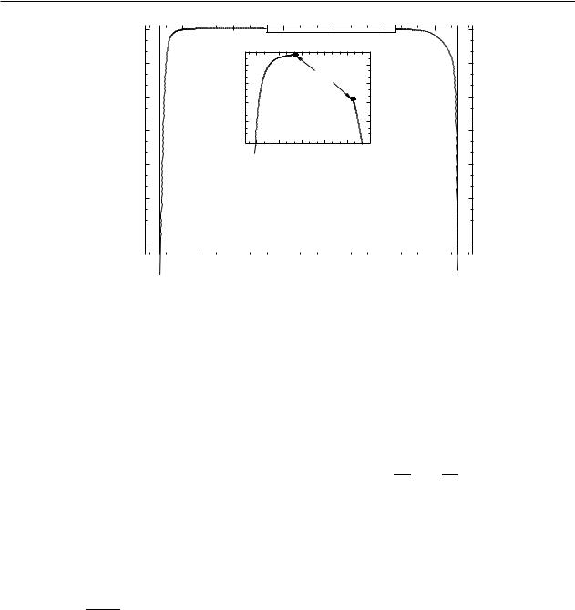
Figure 2 – The total mass of the configuration |
|
|
as a function of the parameter . |
|
|||||||||||||||||
The thin vertical lines correspond to |
|
for |
which the mass of the configurations diverges |
|||||||||||||||||||
|
|
|
|
|
|
|
|
|
|
|
||||||||||||
|
|
|
|
|
|
|
|
|
systems near these points are shown by red lines in figure 1 |
|||||||||||||
(the corresponding solutions describing = crit |
|
|
|
|
|
|
|
|
|
|
|
|
|
|||||||||
with |
|
|
|
for |
= crit1 |
and |
Ω ≈ 0.013 |
for |
= crit2 |
). In the shaded region |
Ω > 1 |
, |
||||||||||
and the solutionsΩ ≈ 0.058 |
|
|
|
|
|
|
|
|
|
|
||||||||||||
for the scalar field are oscillating. The inset shows the region where the masses are close to zero.
For all cases considered here, the throats are
located beyond the fluid, i.e., the fluid is completely |
|||
single- |
|
|
|
hidden in the region between the throats. For other |
|||
values of |
|
one may expect both the existence of |
|
|
throat |
configurations and of systems with |
|
two throats filled with a fluid, as it takes place for the system of Ref. [16] supported by a real scalar field. But this issue requires special studies.
LetusnowconsidertheADMmassoftheabove |
||||||
volume |
|
|
|
|
( ) |
|
systems. For a spherically symmetric configuration, |
||||||
the Misner-Sharp [23] |
mass |
|
inside the |
|||
( ) ≡ |
(2 ) |
= |
1 + (1 + ) |
|||
|
|
Pl |
2 |
0 |
|
|
The Pl |
is the |
|
|
|
||
|
Planck mass. |
|
|
|||
where |
|
|
|
|||
results of the calculations of the mass are presented in figure 2. It is interesting to compare the results obtained with those found for
wormholes supported by a real massless scalar and |
||||||||||
configurations can vary |
|
|
|
|
|
|||||
threaded by the same fluid [16]. Depending on the |
||||||||||
some |
finite posit ve magnitude for |
= 0 |
those |
|||||||
value |
of |
the |
parameter |
|
, masses |
of |
||||
follows |
|
= crit |
|
from 0 (for |
|
) up to |
||||
|
|
|
|
the |
critical |
|||||
|
|
|
|
|
|
|
|
|||
value |
of |
|
|
|
. The |
existence of |
the latter |
|||
|
|
from |
Eq. (15) and corresponds |
to the |
||||||
|
|
|
|
|
|
|
|
||
enclosed by a sphere with circumferential radius |
|||||||||
be defined as follows: |
|
|
|
|
|
> |
|
||
, which corresponds to the center of the system, |
|||||||||
and another sphere having the radius |
|
, can |
|||||||
( ) = |
2 |
4 |
|
0 |
|
2 |
|
|
|
2 |
+ |
2 |
|
0 |
|
|
. |
|
|
Taking the boundary to (spacelike) infinity, the Misner-Sharp mass gives the ADM mass. In the dimensionless variables (9), we then have
− ′2 − Ω2 − 2 − 2 + Λ2 4 2 ′ ′ ,
equality of the denominator to zero; as a result,
|
|
. For the complex scalar fields considered |
|||||
in the present paper, |
we |
have not one but |
two |
||||
→ ∞ |
|
and |
|
, near |
which |
the |
|
critical |
|
values |
|
||||
total |
|
the |
configurations |
increases |
|||
mass of crit1 |
|
crit2 |
|
|
|
||
(modulus) rapidly and eventually diverges (see figure 2). In this case physically interesting
solutions exist |
only for |
|
|
|
and |
|
|||
|
, up/down to the |
values of |
|
for which the |
|||||
|
|
|
> crit1 |
|
< |
||||
boson frequency |
|
|
(see the inset of figure 2). |
||||||
crit2 |
|
there is |
a |
|
|
|
in |
||
Correspondingly, |
discontinuity |
||||||||
|
|
Ω → 1 |
|
|
|
|
|
|
|
16

V. Folomeev et al.
possibleΩvalues> 1 of (the shaded region in figure 2 where ), where only asymptotically oscillating solutionsforthe scalar field do exist [cf. Eq. (17)].
Conclusion
We have considered mixed systems consisting of a complex ghost scalar field with a quartic potential and ordinary polytropic fluid. This study extends the previous researches of Refs. [16, 20] where the systems with a real massless scalar field plus a polytropic fluid [16] and the configurations supported by a complex ghost scalar field without ordinary matter[20]havebeenconsidered.Wehaveshownthat there exist static regular asymptotically flat solutions describing localized configurations in which the fluid is concentrated in a finite-size region. We have demonstrated that for the chosen central value of the scalar field (i) there exist only double-throat configurations; and (ii) the wormhole throats are located outside the fluid (or one can say that the fluid is hidden inside the region between the throats).
Unlike the configurations of Ref. [16], the systems |
|||
two different critical values crit1 |
crit crit2 |
|
|
considered here possess the following new properties: |
|||
(1) Instead of one critical value |
|
, there are |
|
|
and |
|
for |
which the total mass diverges. All regular solutions |
||||||
discontinuity |
|
|
|
|
|
|
possessing finite masses lie in the region between |
||||||
figure 2) where the boson frequency |
|
; this |
||||
these critical |
|
’s, and this region also contains a |
||||
|
in |
|
(shown by the shaded region in |
|||
corresponds to the presence of |
oscillations of the |
|||||
|
Ω > 1 |
|
||||
solutions describing systems |
|
|
|
|||
scalar field, that is physically unacceptable. |
|
|||||
(2) For |
some |
values of |
, there can |
exist |
||
|
|
|
whose fluid density |
|||
and pressure maxima lie not at the center [see figure 1(a)]. This results in the fact that such systems possess two equators resided symmetrically with respect to the center; see figure 1(b).
The solutions obtained cover only a restricted set of the model parameters. In further investigations, we plan to extend these calculations. Moreover, it will be interesting to address their rotating generalizations [24].
Acknowledgements
We are grateful to the Research Group Linkage Programme of the Alexander von Humboldt Foundation for the support of this research. BK and JK gratefully acknowledge support by the DFG Research Training Group 1620 Models of Gravity and the COST Action CA16104.
References
1 Ade P.A.R. et al. (Planck Collaboration) Planck 2015 results. XIII. Cosmological parameters //Astron. Astrophys. – 2016. – Vol.594:A13.
2 Schunck F.E. and Mielke E.W. General relativistic boson stars //Classical Quantum Gravity. – 2003. – Vol. 20. – P.R301. 3 Liebling S.L. and Palenzuela C. Dynamical Boson Stars //Living Rev. Relativity. – 2012. – Vol. 15. – P. 6.
4 Sullivan M. et al.SNLS3: Constraints on Dark Energy Combining the Supernova Legacy Survey Three Year Data with Other Probes //Astrophys. J. – 2011. – Vol.737. – P.102.
5 Dzhunushaliev V., Folomeev V., Myrzakulov R., and Singleton D. Non-singular solutions to Einstein-Klein-Gordon equations with a phantom scalar field //J. High Energy Phys. – 2008. – Vol.7:094. – 14 p.
6 Bronnikov K.A. Scalar-tensor theory and scalar charge //Acta Phys. Polon. – 1973. – Vol.B4. –P.251.
7 Ellis H.G. Ether flow through a drainhole – a particle model in general relativity //Math. Phys. – 1973. – Vol.14. – P.104. 8 Ellis H.G. The Evolving, Flowless Drain Hole: A Nongravitating Particle Model In General Relativity Theory //General
Relativ. Gravit. – 1979. – Vol.10. – P. 105.
9 KodamaT. General RelativisticNonlinear Field:AKink Solution in a GeneralizedGeometry //Phys. Rev. – 1978. – Vol.D18.
– P.3529.
10 Kodama T., de Oliveira L.C.S., and Santos F.C. Properties of a general-relativistic kink solution //Phys. Rev. – 1979. – Vol.D19. – P. 3576.
11 Visser M. Lorentzian Wormholes: From Einstein to Hawking. – New York: Woodbury, 1996. – 412 p.
12 LoboF.S.N. Wormholes, Warp Drives and Energy Conditions. – Springer International Publishing Company, 2017. – 436 p. 13 DzhunushalievV., FolomeevV., KleihausB., and KunzJ. A Star Harbouring a Wormhole at itsCore //J. Cosmol. Astropart.
Phys. – 2011. – Vol.04:031. – 22 p.
14 Dzhunushaliev V., Folomeev V., Kleihaus B., and Kunz J. Mixed neutron star-plus-wormhole systems: Equilibrium configurations //Phys. Rev. – 2012. – Vol.D85:124028. – 14 p.
15 Dzhunushaliev V., Folomeev V., Kleihaus B., and Kunz J. Mixed neutron-star-plus-wormhole systems: Linear stability analysis // Phys. Rev. – 2013. – Vol. D87:104036. – 12 p.
16 Dzhunushaliev V., Folomeev V., Kleihaus B., and Kunz J. Hiding a neutron star inside a wormhole //Phys. Rev. – 2014. – Vol.D89:084018. – 14 p.
17 Aringazin A., Dzhunushaliev V., Folomeev V., Kleihaus B., and Kunz J. Magnetic fields in mixed neutron-star-plus-wormhole systems // JCAP. – 2015. – Vol.1504:005. – 23 p.
17

Mixed star-plus-wormhole systems with a complex scalar field
18 Dzhunushaliev V., Folomeev V., and Urazalina A. Star-plus-wormhole systems with two interacting scalar fields // Int. J. Mod. Phys. – 2015. – Vol.D24. – P.14.
19 Dzhunushaliev V., Folomeev V., Kleihaus B., and Kunz J. Can mixed star-plus-wormhole systems mimic black holes? // JCAP. – 2016. – Vol.1608:030. – 27 p.
20 Dzhunushaliev V., Folomeev V., Kleihaus B., and Kunz J. Wormhole solutions with a complex ghost scalar field and their instability // Phys. Rev. – 2018. – Vol. D97:024002. – 10 p.
21 SalgadoM.,BonazzolaS., GourgoulhonE., and HaenselP. High precisionrotating netronstarmodels 1:Analysis of neutron star properties // Astron. Astrophys. – 1994. – Vol. 291. – P. 155.
22ColpiM., ShapiroS. L.,andWassermanI. BosonStars:GravitationalEquilibriaofSelfinteractingScalarFields//Phys.Rev. Lett. – 1986. – Vol.57. – P.2485.
23 Misner C. W. and SharpD. H. Relativistic equations for adiabatic, spherically symmetric gravitational collapse //Phys. Rev.
– 1964. – Vol.136. – P. B571.
24 Chew X. Y., Dzhunushaliev V., Folomeev V., Kleihaus B., and Kunz J. Rotating wormhole solutions with a complex phantom scalar field // Phys. Rev. – 2019. – Vol. D100:044019. – 12 p.
References
1 P.A.R. Ade et al. (Planck Collaboration), Astron. Astrophys., 594:A13 (2016).
2 Schunck F.E. and Mielke E. W. General relativistic boson stars //Classical Quantum Gravity. – 2003. – Vol. 20. – P.R301. 3 S.L. Liebling and C. Palenzuela, Living Rev. Relativity, 15, 6 (2012).
4 M. Sullivan et al., Astrophys. J., 737, 102 (2011).
5 V. Dzhunushaliev, V. Folomeev, R. Myrzakulov, and D. Singleton, J. High Energy Phys., 7:094 (2008). 6 K.A. Bronnikov, Acta Phys. Polon.B4, 251 (1973).
7 H.G. Ellis, Math. Phys., 14, 104 (1973).
8 H.G. Ellis, General Relativ. Gravit., 10, 105 (1979). 9 T. Kodama, Phys. Rev. D18, 3529 (1978).
10 T. Kodama, L.C.S. de Oliveira, and F.C. Santos, Phys. Rev. D19, 3576 (1979).
11 M. Visser, Lorentzian Wormholes: From Einstein to Hawking, (Woodbury, New York, 1996), 412 p.
12 F.S.N. Lobo Wormholes, Warp Drives and Energy Conditions, (Springer International Publishing Company, 2017), 436 p. 13 V. Dzhunushaliev, V. Folomeev, B. Kleihaus, and J. Kunz, J. Cosmol. Astropart. Phys., 04:031 (2011).
14 V. Dzhunushaliev, V. Folomeev, B. Kleihaus, and J. Kunz, Phys. Rev. D85:124028 (2012). 15 V. Dzhunushaliev, V. Folomeev, B. Kleihaus, and J. Kunz, Phys. Rev. D87:104036 (2013). 16 V. Dzhunushaliev, V. Folomeev, B. Kleihaus, and J. Kunz, Phys. Rev. D89:084018. (2014).
17 A. Aringazin, V. Dzhunushaliev, V. Folomeev, B. Kleihaus, and J. Kunz, JCAP, 1504:005 (2015). 18 V. Dzhunushaliev, V. Folomeev, and A. Urazalina, Int. J. Mod. Phys. D24, 14 (2015).
19 V. Dzhunushaliev, V. Folomeev, B. Kleihaus, and J. Kunz, JCAP, 1608:030 (2016).
20 V. Dzhunushaliev, V. Folomeev, B. Kleihaus, and J. Kunz, Phys. Rev. D97:024002 (2018).
21 M. Salgado, S. Bonazzola, E. Gourgoulhon, and P. Haensel, Astron. Astrophys., 291, 155 (1994). 22 M. Colpi, S.L. Shapiro, and I. Wasserman, Phys. Rev. Lett., 57, 2485 (1986).
23 C.W. Misner and D.H. Sharp, Phys. Rev. 136, B571 (1964).
24 X.Y. Chew, V. Dzhunushaliev, V. Folomeev, B. Kleihaus, and J. Kunz, Phys. Rev. D100:044019 (2019).
18
ISSN1563-0315,еISSN2663-2276 |
RecentContributionstoPhysics.№3(74).2020 |
https://bph.kaznu.kz |
МРНТИ 41.23.29; 41.25.15 |
https://doi.org/10.26577/RCPh.2020.v74.i3.03 |
|
Т. Комеш1,2,3 , А.Б. Манапбаева1
 , Ж. Eсимбек2
 , Н.Ш. Алимгазинова1
 , М.Т. Кызгарина1*
 , Б. Куанбек1
 ,
,
1Казахский национальный университет имени аль-Фараби, Казахстан, г. Алматы, 2Синьцзянская астрономическая обсерватория Академии наук Китая, Китай, г. Урумчи 3Университет академии наук Китая, Китай, г. Пекин
*e-mail: meir83physics@gmail.com
ИНТЕРПРЕТАЦИЯ РАДИОАСТРОНОМИЧЕСКИХ НАБЛЮДЕНИЙ H2CO И H110Α В ОБЛАСТЯХ ЗВЕЗДООБРАЗОВАНИЯ W40
И SERPENS SOUTH МОЛЕКУЛЯРНОГО ОБЛАКA AQUILA
В работе представлены результаты радиоастрономических наблюдений спектральных линий поглощения молекулы формальдегида (H2CO) и рекомбинационной линии H110α в направлении к молекулярному облаку Aquila. Произведена интерпретация радиоастрономических наблюдений H2CO (l10-l11) и H110α в W40 и Serpens South молекулярного комплекса Aquila Rift, которые получены на 26 м радиотелескопе Нань-Шань Синьцзянской астрономической обсерватории Китайской академии наук. Для построения радиокарт были использованы также архивные данные, полученные при наблюдениях молекул 12СО(2−1) и 13CO(2−1) и 6 см континуума для региона Aquila Rift.
На основе полученных наблюдательных данных были рассчитаны оптическая глубина и плотность столбца для линии поглощения H2CO и линии излучения 13CO (J=1–0), построены интегрированные карты интенсивности с областью ионизированного водорода Н II и наложенными контурами, которые соответствуют линиям поглощения H2CO и рекомбинационной линии H110α в направлении молекулярного облака Aquila; карты интенсивности излучения 13CO (1−0), распределения 6 см радиоконтинуума, инфракрасного излучения, наложенные на интегрированные контуры поглощения H2CO; зависимости линейных потоков и пиковых плотностей столбцов для H2CO и 13CO. В работе показано, что регион Serpens South, выделенный контурами при поглощении формальдегида H2CO, происходит от космического микроволнового фона. Была обнаружена корреляция между значениями параметров для линии поглощения H2CO и линии излучения 13CO. Построены интегрированные карты интенсивности при различных значениях скорости канала линии поглощения H2CO в направлении молекулярного облака Aquila. Выявлено, что скорости H2CO и 13CO имеют близкие друг к другу значения.
Анализ проведенного исследования позволил сделать вывод о том, что линии поглощения молекулы формальдегида H2CO и линии излучения 13CO происходят из одного и того же региона в комплексе Aquila Rift молекулярного облака Aquila.
Ключевые слова: молекулярные облака, спектр, звездообразование.
Т. Komesh 1,2,3, A.B. Manapbayeva 1, J. Esimbek 2, N.Sh. Alimgazinova 1, M.T. Kyzgarina1*, B. Kuanbek1
1Al-Farabi Kazakh National University, Kazakhstan, Almaty,
2Xinjiang Astronomical Observatory, Chinese Academy of Sciences, China, Urumqi
3University of the Chinese Academy of Sciences, China, Beijing *e-mail: meir83physics@gmail.com
Interpretation of radioastronomic observations of H2CO and H110α in W40 and Serpens South star formation regions of Aquila molecular cloud
This study presents the results of radio astronomy observations of the absorption spectral lines of a formaldehyde molecule (H2CO) and the H110α recombination line towards the Aquila molecular cloud. The paper interprets the radio astronomy observations of H2CO(l10-l11) and H110α in the W40 and Serpens South of the Aquila Rift molecular complex, which were obtained by the 26m Nan-Shan radio telescope of the Xinjiang Astronomical Observatory of the Chinese Academy of Sciences. In order to construct radio maps, we also used archival data obtained by observing 12СО(2–1) and 13CO(2–1) and 6cm continuum molecules for the Aquila Rift region.
© 2020 Al-Farabi Kazakh National University |
19 |

Интерпретация радиоастрономических наблюдений H2CO и H110α в областях звездообразования W40 ...
Based on the obtained observational data, the optical depth and column density were calculated for the H2CO absorption line and 13CO emission line (J=1–0), integrated intensity maps were constructed with the ionized hydrogen region НII and imposed contours that correspond to the absorption lines of H2CO and the recombination line H110α in the direction of the Aquila molecular cloud; maps of radiation intensity 13CO(1–0), distribution of 6cm of the radio continuum, infrared radiation superimposed on integrated absorption contours of H2CO; dependences of linear flows and peak column densities for H2CO and 13CO are obtained. It is shown that the Serpens South region, highlighted by the contours during the absorption of formaldehyde H2CO, comes from the cosmic microwave background. A correlation was found between the parameter values for the H2CO absorption line and the 13CO emission line. Integrated intensity maps were constructed for various values of the channel velocity of the H2CO absorption line in the direction of the Aquila molecular cloud. It was revealed that the rates of H2CO and 13CO have close values to each other.
An analysis of the study led to the conclusion that the absorption lines of the H2CO formaldehyde molecule and the 13CO emission lines originate from the same region in the Aquila Rift complex of the Aquila molecular cloud.
Key words: molecular clouds, spectrum, star formation.
Т. Көмеш1,2,3, А.Б. Манапбаева1, Ж. Eсiмбeк2, Н.Ш. Алимгазинова1, М.Т. Қызгарина1*, Б. Қуанбек1
1Әл-Фараби атындағы Қазақ ұлттық университеті, Қазақстан, Алматы қ., 2Шыңжаң Астрономиялық Обсерваториясы, Қытай Ғылым Академиясы, ҚХР, Үрімжі қ.
3Қытай Ғылым Академиясы Университеті, ҚХР, Пекин қ. *e-mail: meir83physics@gmail.com
Aquila молекулалық бұлтының W40 және Serpens South жұлдызтүзілу аймақтарындағы H2CO және H110α радиоастрономиялық бақылауларының интерпретациясы
Бұл зерттеуде Aquila молекулалық бұлты бағытындағы формальдегид молекуласының (H2CO) жұтылу спектрлік сызықтарын және H110α рекомбинация сызығын радио астрономиялық бақылау нәтижелері ұсынылды. Мақалада Қытай ғылым академиясының Шыңжаң астрономиялық обсерваториясының 26-метрлік Nanshan радиотелескопында алынған Aquila Rift молекулалық кешенінің W40 және Serpens South H2CO (l10-l11) және H110α астрономиялық бақылаулары түсіндірілді. Радио карталарды салу үшін біз Aquila Rift аймағы үшін 6 см континуум және 12СО(2–1) және 13CO(2–1) молекулаларды бақылау арқылы алынған мұрағаттық деректерді де пайдаландық. Алынған бақылаушылық мәліметтер негізінде H2CO жұтылу сызығы мен 13CO (J=1– 0) сәуле шығару сызығының оптикалық тереңдігі мен бағанның тығыздығы есептелінді, Aquila молекулалық бұлты бағытындағы H2CO жұтылу сызығы мен H110α рекомбинация сызығына сәйкес келетін контурлар салынған және Н II иондалған сутегі аймағы бар интенсивтіліктің қарқындылық картасы құрылды; 13CO (1–0) сәуле шығару қарқындылығының, 6 см радио континуумның таралуы, H2CO жұтылудың интеграцияланған контурлары салынған инфрақызыл сәулеленулер карталары жасалынды; сызықтық ағындар мен шың бағандары тығыздығының тәуелділігі H2CO мен 13CO үшін тұрғызылды. Жұмыста H2CO формальдегидтің жұтылуы кезінде контурлармен ерекшеленген Serpens South аймағы ғарыштық микротолқынды фоннан шығатыны көрсетілді. H2CO жұтылу сызығы мен 13CO сәуле шығару сызығының параметрлік мәндерінің арасында корреляция табылды. Интенсивтіліктің интеграцияланған карталары Aquila молекулалық бұлты бағытында H2CO жұтылу сызығының канал жылдамдығының әртүрлі мәндері үшін құрылды. H2CO мен 13CO жылдамдықтары бір-біріне жақын мәндерге ие екендігі анықталды.
Жүргізілген зерттеуді талдау H2CO формальдегид молекуласының жұтылу сызықтары және 13CO шығарылу сызықтары Aquila молекулалық бұлтының Aquila Rift кешеніндегі бірдей аймақтардан пайда болады деген қорытындыға әкелді.
Түйін сөздер: молекулалық бұлттар, спектр, жұлдызтүзілу.
Введение
Одной из важнейших задач астрофизики является исследование областей и процессов образования звезд. Так как молекулярные облака межзвездной среды Галактики являются важнейшими структурами в областях звездообразования, то изучение их состава, внутреннего
строения, происхождения и эволюции позволит внести существенный вклад в решение данной проблемы.
Молекулярное облако – тип межзвёздного облака, чья плотность и размер позволяют в нём образовываться молекулам и различным сложным соединениям. Молекулы же изза сложной их структуры имеют очень много
20