книги / Разработка нефтяных и газовых месторождений. Ч. 1

2. FORCES ACTING IN RESERVOIR SYSTEMS

2.1. Hydrostatic Pressure Force

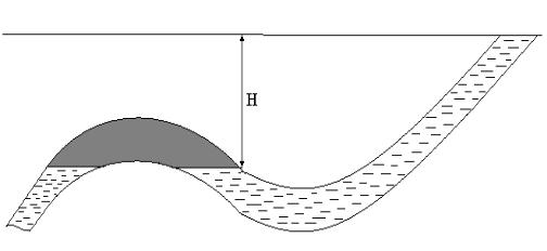
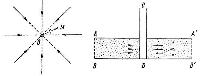
Hydrostatic pressure force depends on edge- (bottom) water drive (fig. 1).

2.1.1. Hydrostatic Pressure of Drilling Mud

One of the most important functions of drilling mud is to create hydrostatic bottomhole pressure required to prevent oil, gas and water ingress and slides.

In fluid at rest, pressure РH is distributed along the depth under the principle equation of hydrostatics:

where РH is total hydrostatic pressure at depth Н (m); Р0 is free fluid surface external pressure; ρ is fluid density; g is gravity acceleration; and Н is well depth.

2.1.2. Reservoir Pressure, Static Level and Reduced Pressure

Pressure (P), under which liquid and gas are in pore (void) space of reservoir (pay formation), is termed reservoir (formation) pressure.

Let us consider a water-saturated reservoir bed (fig. 2). If such reservoir is drilled-in, water inflows the borehole. Two cases are possible:

1)water level raises to some height and stands at height Нst from the center of the reservoir; height Нst is termed static level (Нst ≤ Н); and

2)water overflows at the wellhead (Нst > Н).

22

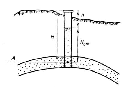
Fig. 2.

In the first case, water pressure in reservoir is balanced by water column pressure in borehole, which, as it is known, is directly proportional to Нst and water density ρw:

where Р is pressure; g is gravity acceleration; С proportionality factor which depends on the taken unit of measurement of Р, Нst, ρw and g.

If Нst is measured in meter (m), Р – Pa, ρw – kg/m3, and g – m/sec2, then С = 1 and we can put down:

If pressure Р is expressed by MPa, fluid density – t/m3, and gravity acceleration is constant magnitude (g = 9.80665 ≈ 9.81 m/sec2), then:

Reservoir pressure before the beginning of reservoir development is termed static (initial) pressure. Reservoir pressure during development is termed dynamic (current) pressure.

Large body of research established that initial pressure of majority of reservoirs depends on depth, hydrostatic pressure and can be determined by formula:

where Рin is initial reservoir pressure, MPa; Н is depth of reservoir point at which pressure is determined, m.

By determining pressure by formula (2.6) at various depths, we obtain the following regularity: pressure is increased on 1 MPa (10 atm) per each 100 meters of depth.

23

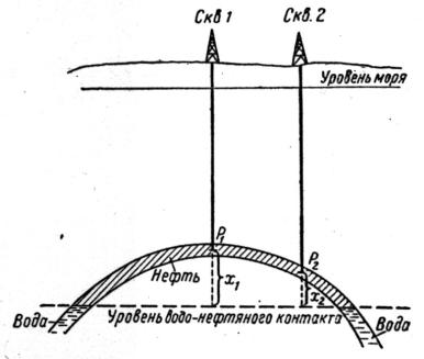
In gas reservoir, reservoir pressure is similar within the entire area or changes insignificantly, and in oil reservoir, at high dip angle, reservoir pressure is different in various parts of reservoir: maximum in wings, and minimum in dome part. That is why pressure change analysis is complicated during reservoir engineering. So, it is more convenient to relate reservoir pressure values to one plane. Very often, the level of initial position of Oil-Water Contact (OWC) is taken as such plane. Reservoir pressure related to such conditional plane is termed reduced pressure.

Fig. 3.

If reservoir pressure in wells 1 and 2 (fig. 3) are, respectively, Р1 and Р2, then, reduced pressure related to the initial level of oil-water contact, is:

where х1 and х2 is distance from the bottomhole to the level of oil-water contact; ρf is reservoir fluid density.

Reduced pressure, converted to any conditional surface (mostly often it is OWC or GOC) is used for pool characteristic.

Often, it is more convenient to use reduced pressure than true pressure. Actually, under real conditions, bottomholes in one and the same reservoir have different hypsometric depths, since, first, reservoirs are penetrated at different depths, and, second, reservoirs are penetrated in various wells at different height.

Due to the above, subsurface pressure gages in bottomhole record various reservoir pressures even under no flow in the reservoir. But, in latter case, all reduced pressures are equal in all wells. And, vice versa, if fluid flows in the reservoir, the reduced pressures are decreased in the direction of the fluid flow.

24

If reference plane is located lower than the middle of the penetrated reservoir, the reduction is made with plus sign, and with minus sign if it located higher than the middle of the penetrated reservoir.

The general formula is as follows:

where Рarp is absolute reservoir pressure; and Z is distance from the middle of the reservoir in the penetration point to the reference plane.

If wellhead is higher than the static fluid level in well (i.e. higher than piezometric level, reservoir pressure can be determined by formula (2.4).

If wellhead is lower than piezometric level, water overflows at wellhead, and reservoir pressure is (see fig. 2.2):

where Рwh is wellhead pressure measured by pressure gage.

2.2. Underground pressure

Underground pressure force depends on weight of overlying rocks. Underground pressure Рundergr can be determined by formula:

where γup is mean specific weight, а ρup is average density of overlying rock with thickness H.

2.3. Fluid and Reservoir Elastic Forces

Elastic properties of fluid and reservoir can be characterized by, respectively, fluid compressibility factor βf and reservoir compressibility factor βr.

Under isometric conditions, the fluid compressibility factor is determined by the following equation:

pressure change.

Fluid volume increases as pressure decreases. By formula (2.11) the fluid compressibility factor is an increment of the unit of fluid volume under pressure decrease on 1 Pa, and is measured by 1/Pа.

Compressibility factor of rock is:

25

Vо ∆P

where indices (о) and (n) correspond to words «rock sample» and «pore»; Vo is initial volume of rock sample; and ∆Vп is pore volume change under pressure change on ∆Р.

In elastic drive theory it is accepted to use more general elastic capacity coefficient (β*), which considers: 1) capacity and elasticity of reservoir and 2) elasticity of fluid saturating this reservoir:

where m is total porosity factor.

As m<<1, value of mβf can be less than βс even if βс < βf. Thus, the effect of reservoir compressibility factor βс on elastic capacity factor β* is not less than the effect of fluid elastic coefficient. For instance, for Tournai carbonate deposits of one of the Permian Prikamie field, for 11 years of development under reduction of reservoir pressure on 11.2 atm (from 17.3 to 16.1 MPa), oil amount, which was obtained due to elastic properties of reservoir, and calculated by formula

amounted to 70.0 thousand m3, which is about 11 % of the accumulated oil production for this period.

2.4. Gas Pressure Force

It is manifested in the form of:

1)expansion of free gas (gas cap) or

2)expansion of oil-dissolved gas.

In nature, under reservoir conditions, gas is always dissolved in oil. As reservoir pressure becomes lower than bubble-point pressure, earlier dissolved gas begins bleeding and continues flowing in the form of bubbles together with oil. As pressure is further decreased, gas is still bleeding, and gas bubble size increases. The formed bubbles of free gas displace fluid from pore space.

2.5. Gravity Force

Oil inflows due to gravity force, if elevation of reservoir drainage zone is higher than elevation of bottomhole.

26

3.CLASSIFICATION OF FILTRATION FLOWS

3.1.Filtration Rate and Flow Rate

Filtration rate (V) is equal to the ratio of volumetric fluid (gas) flow rate (Q) through the cross-sectional area of the given element of porous rock medium to the (F) of normal section of such element in relation to the flow direction:

The notion Filtration Rate makes it possible to consider a reservoir as continuous field of filtration rates and pressures which are, at each point of reservoir, the coordinate function of the given point and time.

The filtration rate differs from the actual fluid or gas rate. To determine the actual flow rate (u), it is necessary to divide the volumetric flow rate Q by area

(S) of the normal cross-sectional area of pore channels of in relation to the flow direction:

where m is porosity factor.

3.2. Filtration Flow Types

Based on the classification by relationship between velocity vector and coordinates, the below types of filtration flow can be singled out:

–one-dimensional flows V = f(x);

–two-dimensional flows V = f(x, y); and

–three-dimensional flows V = f(x, y, z).

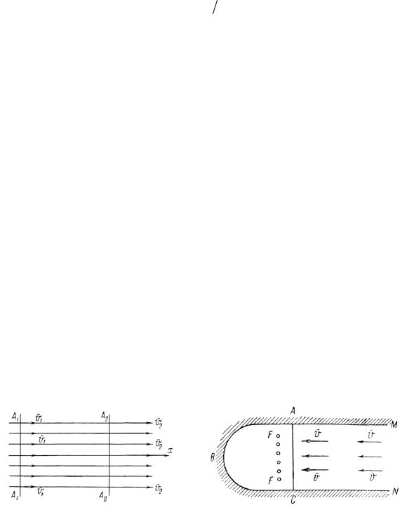
Under one-dimensional flow, the trajectories are composed of parallel straight lines (fig. 4). Flow regularities along all trajectories are the same, so it is sufficient to study flow along one of the trajectories, which can be taken as OX coordinate axis. Position of fluid particle under one-dimensional flow is completely determined by the coordinate axis.

One-dimensional flows are dealt with when fluid or gas flows: 1) through the core in parallel to the core axis in laboratory studies, and 2) fluid flows to well rows (fig. 5) and other.

Two-dimensional flow. Let us assume that under fluid or gas flow in porous rock medium, all particles flow in parallel to one and the same plane. Plane-parallel flow of fluid or gas particles can be termed two-dimensional as, in order to characterize completely such flow, it is sufficient to study such flow even in one plane that is parallel to the main plane; and position of any particle in the particular plane is completely determined by two coordinates. If in each of the above mentioned planes of flow the trajectories are straight lines radially converged at one point (or radiated from one point), such flow is termed twodimensional radial or radial two-dimensional flow. Fig. 6 shows the section of converged radial two-dimensional flow. The condition w = f (r ) is satisfied, i.e. vector of filtration rate is a function of distance (r) from some point (О). The point О is termed discharge or source (flow from the center to periphery).

Tree-dimensional Flow

If all particles of fluid (or gas) flow in porous rock medium so that their filtration rate vectors are not parallel to one and the same plane, such flow is termed spatial or three-dimensional flow. A spatial position of fluid particle is determined by three coordinates. Spherical-radial flow is the specific case of three-dimensional flow (fig. 7).

28

Steady-state and Unsteady-state Flows

Filtration flow is termed stable-state flow if pressure in the given point of reservoir is constant. If pressure in such point is changed in the course of time, such flow is termed unstable-state flow.

For filtration process study, compressible and incompressible fluid flows are distinguished.

4.FILTRATION LAWS

4.1.Linear Filtration Law

The basic ratio of the filtration theory is termed Filtration Law. It establishes relationship between filtration rate vector and pressure field that causes filtration.

Linear filtration law (Darcy law):

where V is filtration rate, ρis fluid density, µ is dynamic viscosity of fluid, ∆P is drawdown, k is proportionality factor which depends on the properties of porous rock medium, and characterizes its ability to deliver fluid and gas under drawdown. Factor k is termed permeability factor which is measured in unit of area.

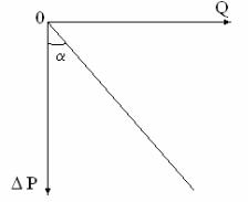
Darcy law (8) is termed Linear Filtration Law as relationship between filtration rate vector (V) and pressure gradient ( ∆P /L) is linear relationship, what is tantamount to linear relationship between drawdown and flow rate:

Fig. 8 provides the indicated line (straight line) that obeys filtration law. Under linear filtration, the production rate (flow rate) is the same under each subsequent unit of drawdown.

Fig. 8. Inflow performance relationship related to incompressible fluid inflow under linear filtration law and water drive

29

4.2. Non-linear Filtration Laws

The general equation of non-linear filtration law is as follows:

index. If n=2, we obtain the non-linear filtration law that is known as Krasnopolskiy non-linear filtration law.

In some cases, for instance, near perforations, filtration rate can increase to the extent that it is impossible to apply Dupuis formula, and, in such cases, binominal formula of inflow should be applied:

The first summand in the equation considers pressure loss due to viscous fluid friction, and the second summand inert component of filtration resistance.

The binominal inflow formula is substantiated and just, in terms of physics, at all Reynolds numbers in petroleum reservoir engineering practice.

30