

1734 |
CHAPTER 22. CONTINUOUS FLUID FLOW MEASUREMENT |
22.8Weighfeeders
A special type flowmeter suited for powdered or granular solids is the weighfeeder. One of the most common weighfeeder designs consists of a conveyor belt with a section supported by rollers coupled to one or more load cells, such that a fixed length of the belt is continuously weighed:
Material from storage bin
Feed chute |
Solid powder or granules |
Load cell |
|
|
Belt motion |
To process |
|
M |
||
|
Motor
The load cell measures the weight of a fixed-length belt section, yielding a figure of material weight per linear distance on the belt. A tachometer (speed sensor) measures the speed of the belt. The product of these two variables is the mass flow rate of solid material “through” the weighfeeder:
W = F v d
Where,
W = Mass flow rate (e.g. pounds per second)
F = Force of gravity acting on the weighed belt section (e.g. pounds) v = Belt speed (e.g. feet per second)
d = Length of weighed belt section (e.g. feet)
22.8. WEIGHFEEDERS |
1735 |
|
A small |
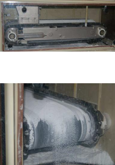
weighfeeder (about two feet in length) is shown in the following photograph, the |
|
weighfeeder |
being used to feed powdered soda ash into water at a municipal filtration plant to |
|
neutralize pH:
In the middle of the belt’s span (hidden from view) is a set of rollers supporting the weight of the belt and of the soda ash piled on the belt. This load cell array provides a measurement of pounds material per foot of belt length (lb/ft).
As you can see in this next picture, the soda ash powder simply falls o the far end of the conveyor belt, into the water below:
1736 |
CHAPTER 22. CONTINUOUS FLUID FLOW MEASUREMENT |
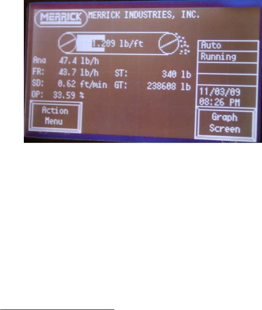
The speed sensor measures belt speed in feet per minute (ft/min). This measurement, when multiplied by the pounds-per-foot measurement sensed by the load cells, translates into a mass flow rate (W ) in units of pounds per minute (lb/min). A simple unit conversion (×60) expresses the mass flow rate in units of pounds per hour (lb/h). A photograph of this weighfeeder’s display screen shows these variables:
Note that the belt loading of 1.209 lb/ft and the belt speed of 0.62 feet per minute do not exactly equate77 to the displayed mass flow rate of 43.7 lb/h. The reason for this discrepancy is that the camera’s snapshot of the weighfeeder display screen happened to capture an image where the values were not simultaneous. Weighfeeders often exhibit fluctuations in belt loading during normal operation, leading to fluctuations in calculated mass flow rate. Sometimes these fluctuations in measured and calculated variables do not coincide on the display screen, given the latency inherent to the mass flow calculation (delaying the flow rate value until after the belt loading has been measured and displayed).
77The proper mass flow rate value corresponding to these two measurements would be 45.0 lb/h.
22.9. CHANGE-OF-QUANTITY FLOW MEASUREMENT |
1737 |
22.9Change-of-quantity flow measurement
Flow, by definition, is the passage of material from one location to another over time. So far this chapter has explored technologies for measuring flow rate en route from source to destination. However, a completely di erent method exists for measuring flow rates: measuring how much material has either departed or arrived at the terminal locations over time.
Mathematically, we may express flow as a ratio of quantity to time. Whether it is volumetric flow or mass flow we are referring to, the concept is the same: quantity of material moved per quantity of time. We may express average flow rates as ratios of changes:
|
|
m |
|
|
|
V |
|
W = |
Q = |
||||||
|
|
|
|||||
t |
t |
||||||
|
|
|
|
|
|||
Where,
W = Average mass flow rate
Q = Average volumetric flow rate m = Change in mass
V = Change in volume t = Change in time
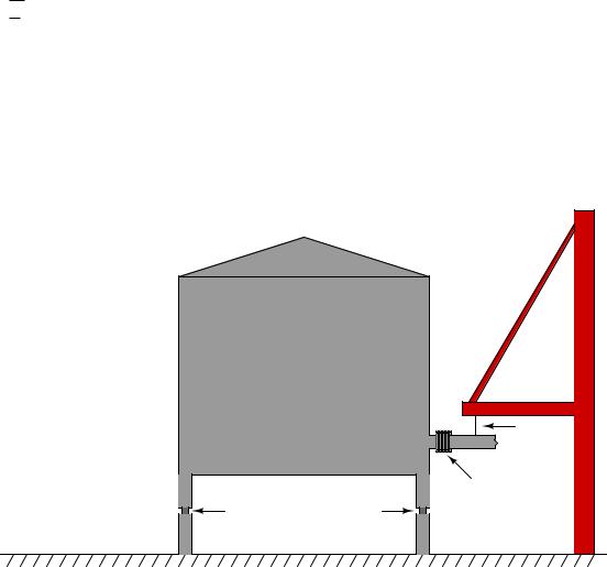
Suppose a water storage vessel is equipped with load cells to precisely measure weight (which is directly proportional to mass with constant gravity). Assuming only one pipe entering or exiting the vessel, any flow of water through that pipe will result in the vessel’s total weight changing over time:
Vessel |
|
Support |
|
|
structure |
|
|
Hanger |
|
|
Pipe |
|
|
Flexible |
Load |
Load |
coupling |
|
||
cell |
cell |
|

1738 |
CHAPTER 22. CONTINUOUS FLUID FLOW MEASUREMENT |
If the measured mass of this vessel decreased from 74688 kilograms to 70100 kilograms between 4:05 AM and 4:07 AM, we could say that the average mass flow rate of water leaving the vessel is 2294 kilograms per minute over that time span.
|
|
m |
= |
70100 kg |
− |
74688 kg |
= |
−4588 kg |
= |
− |
2294 |
kg |
|
W = |
|||||||||||||
t |
4:07 |
− |
4:05 |
2 min |
min |
||||||||
|
|
|
|
|
|
||||||||
|
|
|
|
|
|
|
|
|
|
|
|
||
Note that this average flow measurement may be determined without any flowmeter of any kind installed in the pipe to intercept the water flow. All the concerns of flowmeters studied thus far (turbulence, Reynolds number, fluid properties, etc.) are completely irrelevant. We may measure practically any flow rate we desire simply by measuring stored weight (or volume) over time. A computer may do this calculation automatically for us if we wish, on practically any time scale desired.
Now suppose the practice of determining average flow rates every two minutes was considered too infrequent. Imagine that operations personnel require flow data calculated and displayed more often than just 30 times an hour. All we must do to achieve better time resolution is take weight (mass) measurements more often. Of course, each mass-change interval will be expected to be less with more frequent measurements, but the amount of time we divide by in each calculation will be proportionally smaller as well. If the flow rate happens to be absolutely steady, we may sample mass as frequently as we might like and we will still arrive at the same flow rate value as before (sampling mass just once every two minutes). If, however, the flow rate is not steady, sampling more often will allow us to better see the immediate “ups” and “downs” of flow behavior.
Imagine now that we had our hypothetical “flow computer” take weight (mass) measurements at an infinitely fast pace: an infinite number of samples per second. Now, we are no longer averaging flow rates over finite periods of time; instead we would be calculating instantaneous flow rate at any given point in time.
Calculus has a special form of symbology to represent such hypothetical scenarios: we replace the Greek letter “delta” (Δ, meaning “change”) with the roman letter “d” (meaning di erential ). A simple way of picturing the meaning of “d” is to think of it as meaning an infinitesimal change in whatever variable follows the “d” in the equation78. When we set up two di erentials in a quotient,
we call the d |
fraction a derivative. Re-writing our average flow rate equations in derivative (calculus) |
||||
d |
|
|
|
|
|
form: |
|
|
|
|
|
|
W = |
dm |
Q = |
dV |
|
|
dt |
dt |
|||
|
|
|
|||
Where,
W = Instantaneous mass flow rate
Q = Instantaneous volumetric flow rate
dm = Infinitesimal (infinitely small) change in mass dV = Infinitesimal (infinitely small) change in volume dt = Infinitesimal (infinitely small) change in time
78While this may seem like a very informal definition of di erential, it is actually rooted in a field of mathematics called nonstandard analysis, and closely compares with the conceptual notions envisioned by calculus’ founders.
22.9. CHANGE-OF-QUANTITY FLOW MEASUREMENT |
1739 |
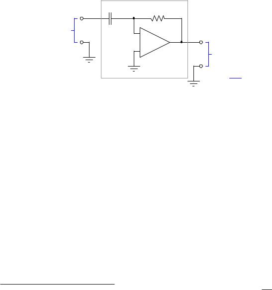
We need not dream of hypothetical computers capable of infinite calculations per second in order to derive a flow measurement from a mass (or volume) measurement. Analog electronic circuitry exploits the natural properties of resistors and capacitors to essentially do this very thing in real time79:
|
|
Differentiator circuit |
|
C |
R |
|
|
|
Voltage signal |
|
|
in from mass |
|
− |
transmitter |
|
|
m |
|
+ |
|
|
Voltage signal out representing mass flow rate
dm
dt
In the vast majority of applications you will see digital computers used to calculate average flow rates rather than analog electronic circuits calculating instantaneous flow rates. The broad capabilities of digital computers virtually ensures they will be used somewhere in the measurement/control system, so the rationale is to use the existing digital computer to calculate flow rates (albeit imperfectly) rather than complicate the system design with additional (analog) circuitry. As fast as modern digital computers are able to process simple calculations such as these anyway, there is little practical reason to prefer analog signal di erentiation except in specialized applications where high speed performance is paramount.
Perhaps the single greatest disadvantage to inferring flow rate by di erentiating mass or volume measurements over time is the requirement that the storage vessel have only one flow path in and out. If the vessel has multiple paths for liquid to move in and out (simultaneously), any flow rate calculated on change-in-quantity will be a net flow rate only. It is impossible to use this flow measurement technique to measure one flow out of multiple flows common to one liquid storage vessel.
A simple “thought experiment” confirms this fact. Imagine a water storage vessel receiving a flow rate in at 200 gallons per minute. Next, imagine that same vessel emptying water out of a second pipe at the exact same flow rate: 200 gallons per minute. With the exact same flow rate both entering and exiting the vessel, the water level in the vessel will remain constant. Any change-of-quantity flow measurement system would register zero change in mass or volume over time, consequently calculating a flow rate of absolutely zero. Truly, the net flow rate for this vessel is zero, but this tells us nothing about the flow in each pipe, except that those flow rates are equal in magnitude and opposite in direction.
79To be precise, the equation describing the function of this analog di erentiator circuit is: Vout = −RC dVdtin . The negative sign is an artifact of the circuit design – being essentially an inverting amplifier with negative gain – and not an essential element of the math.
1740 |
CHAPTER 22. CONTINUOUS FLUID FLOW MEASUREMENT |
22.10Insertion flowmeters
This section does not describe a particular type of flowmeter, but rather a design that may be implemented for several di erent kinds of flow measurement technologies. When the pipe carrying process fluid is large in size, it may be impractical or cost-prohibitive to install a full-diameter flowmeter to measure fluid flow rate. A practical alternative for many applications is the installation of an insertion flowmeter: a probe that may be inserted into or extracted from a pipe, to measure fluid velocity in one region of the pipe’s cross-sectional area (usually the center).
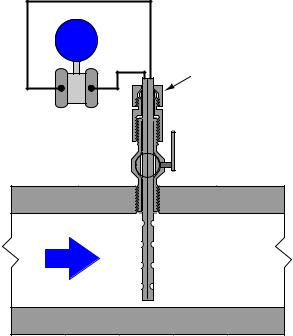
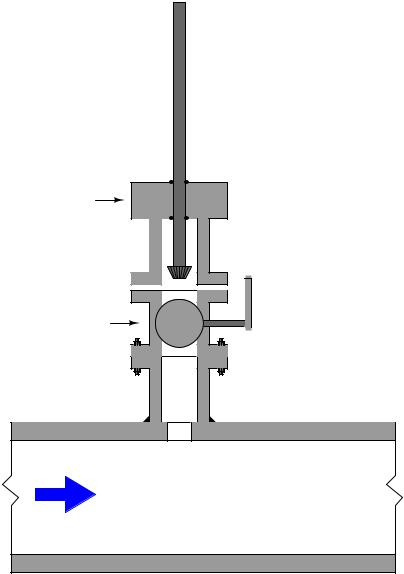
A classic example of an insertion flowmeter element is the Annubar, a form of averaging pitot tube pioneered by the Dieterich Standard corporation. The Annubar flow element is inserted into a pipe carrying fluid where it generates a di erential pressure for a pressure sensor to measure:
L |
H |
Compression nut |
|
("Gland" nut) |
|||
|
|
||
|
|
Handle |
|
|
Ball valve |
|
|
Pipe wall |
Pipe wall |
||
Flow
Pipe wall
22.10. INSERTION FLOWMETERS |
1741 |
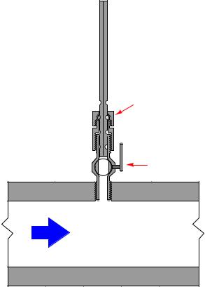
The Annubar element may be extracted from the pipe by loosening a “gland nut” and pulling the assembly out until the end passes through a hand ball valve. Once the element has been extracted this far, the ball valve may be shut and the Annubar completely removed from the pipe:
|
Loosen this nut to |
|
|
extract the Annubar |
|
Ball valve |
Close this ball valve |
|
when the Annubar is clear |
||
|
||
Pipe wall |
Pipe wall |
Flow
Pipe wall
For safety reasons, a “stop” is usually built into the assembly to prevent someone from accidently pulling the element all the way out with the valve still open.
1742 |
CHAPTER 22. CONTINUOUS FLUID FLOW MEASUREMENT |
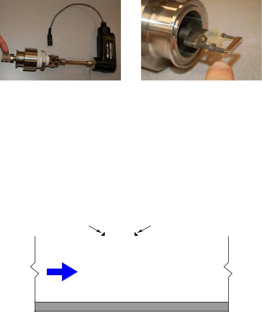
Other flowmeter technologies manufactured in insertion form include vortex, turbine, and thermal mass. An insertion-type turbine flowmeter appears in the following photographs:
If the flow-detection element is compact rather than distributed (as is certainly the case with the turbine flowmeter shown above), care must be taken to ensure correct positioning within the pipe. Since flow profiles are never completely flat, any insertion meter element will register a greater flow rate at the center of the pipe than near the walls. Wherever the insertion element is placed in the pipe diameter, that placement must remain consistent through repeated extractions and re-insertions or else the e ective calibration of the insertion flowmeter will change every time it is removed and re-inserted into the pipe. Care must also be taken to insert the flowmeter so the flow element points directly upstream, and not at an angle.
A unique advantage of insertion instruments is that they may be installed in an operating pipe by using specialized hot-tapping equipment. A “hot tap” is a procedure whereby a safe penetration is made into a pipe while the pipe is carrying fluid under pressure. The first step in a hot-tapping operation is to weld a “saddle tee” fitting on the side of the pipe:
|
|
|
|
|
|
|
Weld |
|
|
|
|
Weld |
|
|
|
|
|
|
|
|
|
|
|
|
|
|
|
Fluid
22.10. INSERTION FLOWMETERS |
1743 |
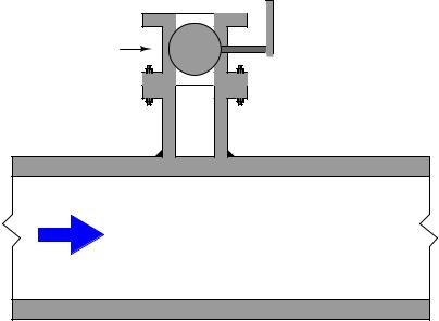
Next, a ball valve is bolted onto the saddle tee flange. This ball valve will be used to isolate the insertion instrument from the fluid pressure inside the pipe:
Ball valve
Fluid
1744 |
CHAPTER 22. CONTINUOUS FLUID FLOW MEASUREMENT |
A special hot-tapping drill is then bolted to the open end of the ball valve. This drill uses a high-pressure seal to contain fluid pressure inside the drill chamber as a motor spins the drill bit. The ball valve is opened, then the drill bit is advanced toward the pipe wall where it cuts a hole into the pipe. Fluid pressure rushes into the empty chamber of the ball valve and hot-tapping drill as soon as the pipe wall is breached:
High-pressure seals
Hot-tapping |
drill motor |
Ball valve |
(open) |
Drill bit |
Fluid |
22.10. INSERTION FLOWMETERS |
1745 |
Once the hole has been completely drilled, the bit is extracted and the ball valve shut to allow removal of the hot-tapping drill:
Hot-tapping
drill motor
Ball valve (shut)
Fluid
Now there is a flanged and isolated connection into the “hot” pipe, through which an insertion flowmeter (or other instrument/device) may be installed.
Hot-tapping is a technical skill, with many safety concerns specific to di erent process fluids, pipe types, and process applications. This brief introduction to the technique is not intended to be instructional, but merely informational.