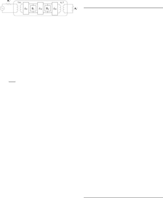
Fig. 3 Model of a coupled-resonator circuit with normalized termination resistances

Table 1 Theoretical values of the design parameters for the filterantenna module at 2 GHz

The normalized termination resistances obtained after

where R1 and R2 are the real termination resistances, and L1 and L2 are the auto-inductances of the input and output resonator, respectively.

The external quality factor, by definition, is given by:

Combining the definition in (11) with (10), the input and

The coupling coefficient k12 is readily obtained from the coupling matrix. The coupling matrix (M0) of a prototype coupledresonator circuit, obtained with (8), is transformed into the coupling matrix (M) of the real

The coupling coefficient k12 is the value of the two elements on the diagonal of the coupling matrix M, which must be the same, because of the symmetry of this matrix:

In this manner, the three design parameters are obtained by using (12) and (14).

For the filter-antenna module at 2 GHz, the input parameters to the synthesis procedure were:

•N = 2

•f0 = 1.960 GHz

•-3 dB FBW = 4.23 %

•RL = 13.10 dB

•Transmission zeros (for the prototype bandpass response): -2.8 and 1.4 rad/s. These fictitious transmission zeros produce reflection zeros at 1.947 and 1.998 GHz.

The obtained values for the design parameters are presented in Table 1.

On the other hand, for the filter-antenna module at 5 GHz, the input parameters to the synthesis procedure were:

•N = 2

•f0 = 4.954 GHz

•-3 dB FBW = 4.42 %

•RL = 10.96 dB

•Transmission zeros (for the prototype bandpass response): -1.4 and 3.2 rad/s. These fictitious transmission zeros produce reflection zeros at 4.846 and 4.987 GHz.

The obtained values for the design parameters are presented in Table 2.

3.2 Characterization of the design parameters

The second stage of the design procedure consists of characterizing the design parameters (QE-in, k12 and QE-out) as a function of the physical dimensions that control them. This characterization is presented in [9] and the details are discussed below.

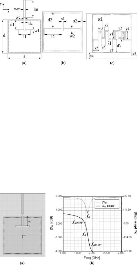
The physical dimensions of the filter-antenna module are presented in Fig. 4.

The input external quality factor (QE-in) depends on all the dimensions of the access line (Fig. 4(a)), the coupling coefficient (k12) mainly depends on the dimensions d2, l2 and w2 of the inter-cavity slots (Fig. 4(b)), and the output external quality factor (QE-out) depends on all the dimensions of the meandered slots (Fig. 4(c)). However, the access line dimensions required to accomplish a good energy coupling at the input of the cavity have been established in previous works [10]. Likewise, the meandered slots dimensions required to allow the radiation of

Table 2 Theoretical values of the design parameters for the filterantenna module at 5 GHz

the antenna have been established in [5]. Hence, for the purpose of characterization, just one of the access line dimensions and one of the meandered slots dimensions are chosen to perform the characterization procedure of QE-in and QE-out, respectively. The chosen dimensions are those that most affect the value of these two parameters. These dimensions are: the position of the access slot (d1 in Fig. 4(a)) for the characterization of QE-in and the position of the meandered slots (d3 in Fig. 4(c)) for the characterization of QE-out. Otherwise, in order to completely describe the inter-cavity coupling proposed in this paper, it was characterized as a function of the three variables d2, l2 and w2 (Fig. 4(b)). After this characterization, it was noticed that the dimension that most affects the value of k12 is the position of the inter-cavity slots (d2). Thus, it was the selected variable to perform the characterization of this design parameter. The other variables of the inter-cavity slots were set at the value that best allows the establishment of the field distribution required for the antenna’s radiation.

The characterization of the design parameters QE-in, k12 and QE-out as a function of the dimensions d1, d2 and d3, respectively, is presented below.

Fig. 5 Characterization of the input external quality factor (QE-in). a Simulated structure. b Simulated S11 parameter

3.2.1Characterization of the input external quality factor

(QE-in)

The characterization method for QE-in was taken from [11]. This method is based on the simulated magnitude and phase of the S11 parameter corresponding to the input cavity with the access line to be characterized (Fig. 5(a)). The coupling of the input cavity, with the other resonator must be eliminated. So, the inter-cavity slots were covered by a perfect ground plane. The full-wave simulation was done in Ansoft HFSS. The obtained S11 parameter, in magnitude and phase, is presented in Fig. 5(b). Over the curves of this parameter, three frequencies are determined, as shown in Fig. 5(b): the resonance frequency (f0), the frequency for which the S11 phase is 90L higher than the phase at central frequency (fu0?90L) and the frequency for which the S11 phase is 90L lower than the phase at central frequency (fu0–90L).

With these three frequencies, the value of the input external quality factor is determined, by using (15).

Table 3 Characterized values of QE-in as a function of the dimension d1 and frequencies used in the computation (filter-antenna module at 2 GHz)

Table 4 Characterized values of QE-in as a function of the dimension d1 and frequencies used in the computation (filter-antenna module at 5 GHz)

The procedure is repeated for different values of the dimension d1. The characterization results are presented in Tables 3 and 4, for the 2 GHz and the 5 GHz filter-antenna module, respectively.

The third stage of the design procedure consists of crossing the values of Q obtained theoretically (Tables 1, 2) and the curves obtained after the characterization procedure, formed by interpolation of the values presented in Tables 3 and 4. This is done for both filterantenna modules, at 2 and 5 GHz, in Fig. 6.

From Fig. 6, the value of the physical dimension d1 for obtaining the desired QE-in can be determined. This value is presented in Table 5 for both filter-antenna modules.

This way, the design procedure is complete with respect to the design parameter QE-in.

3.2.2 Characterization of the coupling coefficient (k12)

The characterization method was developed from (16), taken from [11]. This expression allows the computation of the coupling coefficient of a coupled-resonator circuit

In (16), f01 and f02 are the auto-resonance frequencies of the input and output resonator, respectively, while f1 and f2 are the eigen-frequencies of the full resonant structure.

Fig. 6 Characterization curve for QE-in (continuous line) crossed with the theoretical value (dashed line). a For the filter-antenna module at 2 GHz. b For the filter-antenna module at 5 GHz

Table 5 Values of the dimension d1 required to obtain the desired

QE-in

In order to determine the auto-resonance frequencies, f01 and f02, the input and output cavities were simulated separately. The input cavity was completely closed with a perfect ground plane, while the meandered slots were kept at the lower metallization of the output cavity. The used meandered slots were previously designed in order to allow the radiation. Both cavities were fed by means of a plane wave, internal to the structure, and the auto-resonance frequencies were determined as the frequencies for which the magnitude of the electric field, observed at different points, was maximized. The obtained values for these frequencies are presented in Table 6, for the filter-antenna modules at 2 and 5 GHz.

The eigen-frequencies of the full resonant structure were determined after coupling the input and ouput cavities by means of the inter-cavity slots. The S11 parameter of this structure was simulated in Ansoft HFSS, by using the access line designed in the previous sub-section in order to obtain the required QE-in. The two eigen-frequencies were

Table 6 Auto-resonance frequencies of the input and output cavities of the proposed filter-antenna modules at 2 and 5 GHz

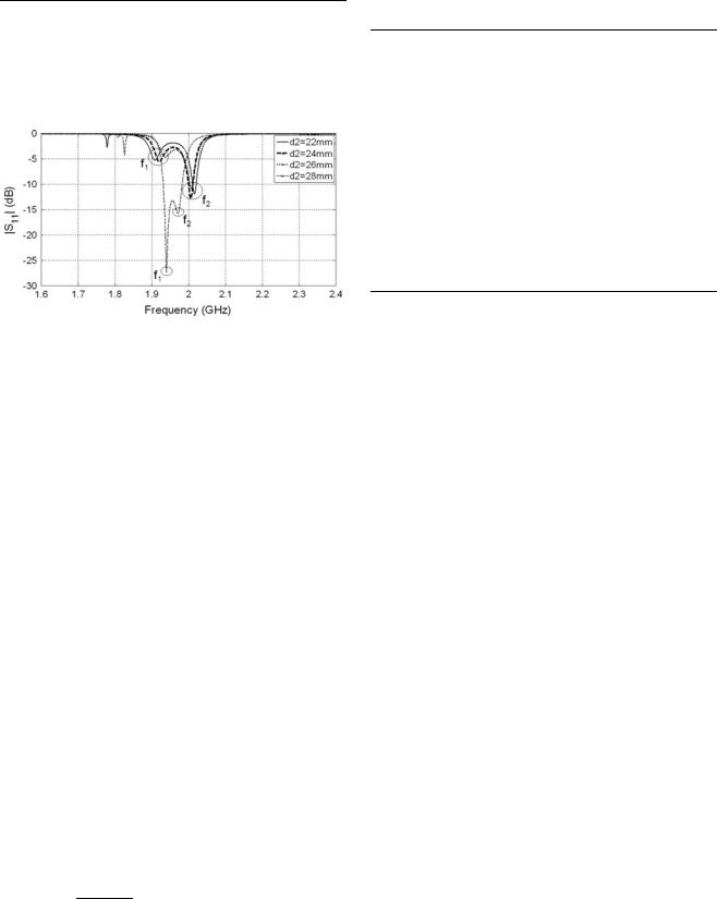
Fig. 7 Determination of the eigen-frequencies (f1, f2) as the frequencies where the two reflection zeros appear in the bandpass region

determined as the frequencies where the reflection zeros are obtained, in the magnitude of the S11 parameter, in the bandpass region, as shown in Fig. 7. The physical dimension used for the characterization procedure is the position of the inter-cavity slots (d2). The other dimensions of these slots were set at the value that best allows the establishment of the field distribution required for antenna’s radiation, as stated before.

For the filter-antenna module at 2 GHz, the different pairs of eigen-frequencies, obtained for each value of the dimension d2, are presented in Table 7, as well as the value of k12 computed from (16), by using the auto-resonance frequencies of Table 6. The same results are presented for the filter-antenna module at 5 GHz in Table 8.

The third stage of the design procedure, consisting of crossing the theoretical values of k12 (Tables 1, 2) with the characterized values that have been just found (Tables 7, 8), is done in Fig. 8, for both filter-antenna modules.

The values of the dimension d2 required to obtain the theoretical k12 can be established from Fig. 8. These values are presented in Table 9.

3.2.3Characterization of the output external quality factor

(QE-out)

For this characterization procedure, the definition (17) of the output external quality factor was used [14]:

Table 7 Characterized values of k12 as a function of the dimension d2, computed from the presented eigen-frequencies (f1 and f2) and from the auto-resonance frequencies f01 = 1.932 GHz and f02 = 2.047 GHz (filter-antenna module at 2 GHz)

Table 8 Characterized values of k12 as a function of the dimension d2, computed from the presented eigen-frequencies (f1 and f2) and from the auto-resonance frequencies f01 = 4.919 GHz and f02 = 5.147 GHz (filter-antenna module at 5 GHz)

Fig. 8 Characterization curve for k12 (continuous line) crossed with the theoretical value (dashed line). a For the filter-antenna module at 2 GHz. b For the filter-antenna module at 5 GHz

Table 9 Values of the dimension d2 required to obtain the desired k12

In this definition, x0 is the central frequency of the filter-antenna module, Wm and We are the average stored energies in the output cavity, of magnetic and electric type,

where l and e are the medium permeability and permittivity, respectively, and H and E are the intensities of magnetic and electric field, respectively.

On the other hand, in (17) Prad is the power radiated by the slot antenna of the output cavity. This power is given by the expression below [15].

where Sav is the average power density calculated as one half of the real part of the Poynting vector [15].

The quantities Wm, We and Prad are calculated through (18)–(20), by using the ‘‘HFSS Fields Calculator’’ tool of Ansoft HFSS. It is done for different positions of the meandered slots (physical dimension d3 in Fig. 4(c)). The central frequency x0 is the same used for the extraction of the theoretical values of the design parameters (Sect. 3.1.3): 1.960 GHz for the filter-antenna module at 2 and 4.954 GHz for the module at 5 GHz.

The so obtained values of Wm, We and Prad, as well as the corresponding value of QE-out calculated from them, are presented in Tables 10 and 11, for the filter-antenna modules at 2 and 5 GHz, respectively.

In order to complete the third-stage of the design process, the interpolated characterization curves obtained from Tables 10 and 11 are crossed with the required theoretical values of QE-out (Tables 1, 2), as shown in Fig. 9 for both filter-antenna modules.

The value of d3 required to obtain the theoretical value of QE-out is extracted from Fig. 9 and presented in Table 12, for both filter-antenna modules.

Table 10 Characterized values of QE-out as a function of d3, and values of the quantities Wm, We and Prad used for its computation (filter-antenna module at 2 GHz)

Table 11 Characterized values of QE-out as a function of d3, and values of the quantities Wm, We and Prad used for its computation (filter-antenna module at 5 GHz)

Fig. 9 Characterization curve for QE-out (continuous line) crossed with the theoretical value (dashed line). a For the filter-antenna module at 2 GHz. b For the filter-antenna module at 5 GHz