


5
Magnetic Resonance Spectroscopy
5.1 Introduction
Focus Point
•MRS can be considered as a bridge between the anatomic and physiological information and the metabolic characteristics of tissue in vivo.
•The principal phenomenon of MRS is the “chemical shift,” which is directly related to the biochemical environment of every nucleus.
•The proton nucleus is the most useful nucleus for MRS, due to its high natural abundance (>99.9%) and intrinsic sensitivity (high gyromagnetic ratio γ).
Magnetic resonance spectroscopy (MRS) is a technique which provides a non-invasive method for characterizing the cellular biochemistry of brain pathologies, as well as for monitoring the biochemical changes after treatment in vivo. In that sense, it can be considered a bridge between the anatomical and physiological information and the metabolic characteristics of tissue in vivo (Soares and Law, 2009).
The principal phenomenon is the so-called “chemical shift,” which is caused by the unique (for every nucleus) shielding from the external magnetic field (B0) by the electrons surrounding them. Hence, this chemical shift effect is directly related to the biochemical environment of the nuclei. The electron magnetic moment opposes the primary applied magnetic field B0; therefore, the more the electrons the less the magnetic field the nuclei will “feel.” This “feeling” can be expressed as the effective magnetic field Bn of the nucleus:
Bn = B0 (1− σ) |
(5.1) |
where σ, is the screening constant, which is proportional to the chemical environment of the nucleus. Hence, in vivo MRS is a combination of MR imaging and chemical spectroscopy, where instead of an image, a spectrum of resonant peaks is produced.
Due to the chemical shift phenomenon, it is evident that MRS is feasible on any nucleus possessing a magnetic moment, such as a proton (1H), carbon-13 (13C), phosphorus (31P), and sodium (23Na).
Early MRS studies were focused on the phosphorus nucleus (31P) since this was the most technically feasible at the early 1980s when in vivo MRS became possible (Luyten et al., 1989). In recent years, though, proton MRS (1H-MRS) has become much more popular as it is possible to obtain high resolution spectra in reasonably short scan times (Frahm et al., 1989; Soares and Law, 2009) due to proton’s high natural abundance (>99.9%) and intrinsic sensitivity (high
91
92 |
Advanced MR Neuroimaging: From Theory to Clinical Practice |
gyromagnetic ratio γ). Until now, 1H-MRS has been used both as a research as well as a clinical tool for detecting abnormalities, visible or not yet visible, on conventional MRI. Suggestively, Möller-Hartman et al. reported that when only the MR images were used for radiological diagnosis of focal intracranial mass lesions, their type and grade were correctly identified in 55% of the cases. The addition of MR spectroscopic information significantly increased the proportion of correctly diagnosed cases to 71% (Möller-Hartmann et al., 2002).
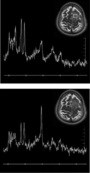
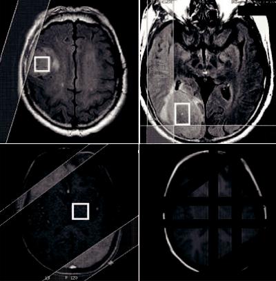
Figure 5.1 illustrates typical examples of magnetic resonance spectra of a 62-year old male with a glioma from (a) the lesion and (b) the contralateral normal parenchyma. The detection
AH
LA
4 3 2 1 0 PF
(a) AH
LA
4 3 2 1 0
PF
(b)
FIGURE 5.1 Typical example of single voxel magnetic resonance spectroscopy of a 62-year-old male with a glioma. (a) Spectrum from the lesion. (b) Spectrum from the contralateral normal parenchyma.

Magnetic Resonance Spectroscopy |
93 |
of spatial or signal abnormalities as a result of the disease conditions is evident by pure visual evaluation of the spectra.
The application of 1H-MRS has been always challenging in terms of its technical requisites (field homogeneity, gradients, coils and software), as well as the accurate metabolic interpretation with regard to pathological processes. Despite the challenges, the clinical applications of 1H-MRS are continuously increasing as the clinical hardware has become more robust and user-friendly along with improved data analysis, spectra post-processing techniques and metabolite interpretation confidence.
The success of MRS as a valuable clinical tool depends on the accuracy of the acquired data as well as correct post-process and analyses. The purpose of this chapter is to elaborately introduce the current status of 1H-MRS in terms of the metabolites detected in the brain with their clinical usefulness, including the technical considerations, the acquisition, and postprocessing methods.
5.2 MRS Basic Principles Explained
Focus Point
•The position of the peaks denotes frequency and determines certain metabolite presence based on their chemical shift.
•The area under the peak is roughly proportional to the concentration of metabolites.
•The ppm unit represents frequencies as a fraction of their absolute resonance frequency, and is independent of field strength.
Proton, derived from the Greek word πρώτον (meaning “first”) is a subatomic particle with a positive electric charge and one-half spin, and exhibits the electromagnetic properties of a dipole magnet. This name was given to the hydrogen nucleus by Ernest Rutherford in 1920.
When protons are placed in an external magnetic field B0, they align themselves along the direction of the field (either parallel or anti-parallel) and demonstrate a circular oscillation. The frequency of this circular motion (called Larmor frequency) is dependent on the strength of the local magnetic field and the molecular structures to which protons belong. This can be expressed by the Larmor equation:
ω0 = γ B0 |
(5.2) |
where ω0 is the Larmor frequency, γ is the gyromagnetic ratio specific for the nucleus, and B0 is the strength of the external magnetic field.
When a RF pulse (in other words electromagnetic energy) is supplied at this frequency, the molecules absorb this energy and change their alignment. When the RF pulse is switched off, the molecules realign themselves to the magnetic field by releasing their absorbed energy. This released energy is the basis of the MR signal and hence MR imaging.
Proton MRS, or 1H-MRS, uses the same hardware as conventional MRI, however, the main difference is that the frequency of the MR signal is used to encode different types of information. MRI generates structural images, whereas 1H-MRS provides chemical information about the tissue under study. The MRS technique also uses gradients to selectively excite a particular volume of tissue (a so-called voxel), but rather than creating an image of it, it records the free induction decay (FID) and produces a spectrum from that voxel.
94 |
|
Advanced MR Neuroimaging: From Theory to Clinical Practice |
||
|
|
Volunteer |
|
Phantom |
|
|
|
|
NAA |
|
|
NAA |
|
|
|
Cr |
|
Cr |
|
|
|
Cho |
|
|
|
|
|
|
|
|
Cho |
|
|
|
ml |
Glx |
Lipids + Lactate |
|
|
|
|
|
||
|
|
ml |
Glx |
Lipids + Lactate |
4 |
3 |
2 |
1 |
0 |
4 |
3 |
2 |
1 |
0 |
FIGURE 5.2 Left: 1H-MRS spectrum from the white matter (WM) measured at 3T in the brain of a 19-year-old healthy volunteer. Right: Spectrum from a standard spectroscopy phantom (25-cm-diameter MRS HD sphere; General Electric Company). The metabolites in the phantom are 3.0 mmol/L choline chloride, 10.0 mmol/L creatine hydrate, 12.5 mmol/L N-acetylaspartic acid, 7.5 mmol/L myo-inositol, 12.5 mmol/L L-glutamic acid, and 5 mmol/L lactate, containing 0.1% sodium azide, 0.1% Magnavis, 50 mmol/L potassium dihydrogen phosphate, and 56 mmol/L sodium hydroxide. PRESS, TE = 35 ms, TR = 1500 ms, voxel size 20 × 20 × 20 mm3, 128 signal averages.
Figure 5.2 illustrates a 1H-MRS spectrum from the white matter (WM) of a 19-year-old healthy volunteer measured at 3T (left) and (right) a spectrum from a standard spectroscopy phantom (25-cm-diameter MRS HD sphere; General Electric Company).
The vertical axis (y) represents the signal intensity or relative concentration for the various cerebral metabolites and the horizontal axis (x) represents the chemical shift frequency in parts per million (ppm). ppm is commonly used instead of frequency in Hz because the ppm unit represents frequencies as a fraction of their absolute resonance frequency, and is independent of field strength. Hence spectra originating from different magnet strengths (e.g., 1.5T vs. 3T) can be directly compared.
The nature of the chemical shift effect is to produce a change in the resonant frequency for nuclei of the same type attached to different chemical species. The phenomenon is due to variations in surrounding electron clouds of neighboring atoms, which shield nuclei from the main magnetic field (B0). The resulting frequency difference can be used to identify the presence of important chemical compounds.
In other words, metabolites can be differentiated based on their slightly different resonant frequencies due to their different local chemical environments. This separation (i.e., the chemical shift) is depicted as a ppm difference on the horizontal axis of spectra.
The only pre-requirement is that the water peak must be suppressed so that the relatively low concentration metabolites (about four orders of magnitude lower) can be evaluated.
In Figure 5.2 it can be noticed that 0 ppm is on the right-hand side and that the x-axis limit is 4 ppm. That is because above 4 ppm the suppression of the water peak (more specifically at 4.7 ppm) makes the neighboring portions of the spectrum unreliable. It must also be noted that

Magnetic Resonance Spectroscopy |
95 |
the phantom spectrum of Figure 5.2 (right) has been corrected for temperature. The signal is inversely proportional to the absolute temperature of the tissue or the object under evaluation (Kreis, 1997). As the temperature is reduced, the Boltzmann distribution gives a larger difference between spin populations, and hence the magnetization of the sample increases (Hoult and Richards, 1976).Hence, the phantom temperature, which is about 20° Celsius (at scanner room temperature) causes a shift in the spectrum of about 0.1 ppm to the right and needs to be corrected for in order to compare spectra.
Within the spectrum, metabolites, due to the chemical shift effect, are characterized by one or more peaks with a certain resonance frequency, line width (full width at half maximum of the peak’s height, FWHM), line shape (e.g., Lorentzian or Gaussian), phase, and peak area according to the number of protons that contribute to the observed signal. By monitoring those peaks, 1H-MRS can provide a qualitative and/or a quantitative (provided there is adequate signal post-processing) analysis of a number of metabolites within the brain if a reference of known metabolite concentration is used at a particular field strength (Christiansen et al., 1993; Jansen et al., 2006; Sarchielli et al., 1999; Sibtain et al., 2007). Generally, the relative areas under each peak are roughly proportional to the number of nuclei in that particular chemical environment.
5.2.1 Technical Issues
Focus Point
•Increased field strength (B0):
•Increased B0 increases SNR and chemical shift leading to improved spectral resolution and better visualization of the weakly represented neurochemicals.
•Comes with a price tag: increased spatial misregistration and magnetic susceptibility of the paramagnetic materials.
•Shimming:
•The process of optimizing the magnetic field homogeneity over the ROI. Efficient shimming results in improved spectral resolution.
•Voxel positioning:
•Cautious spatial localization of the voxel removes unwanted signals from outside the ROI and avoids partial volume effects.
•Voxel size:
•A practical minimum for the voxel size in in-vivo MRS is 1 cm3.
5.2.2 Data Acquisition
In order to acquire high quality spectra, several technical considerations should be taken into account concerning the available MRS techniques, the applied magnetic field, the shimming procedures, as well as the good control of the spatial origin of the spectra.
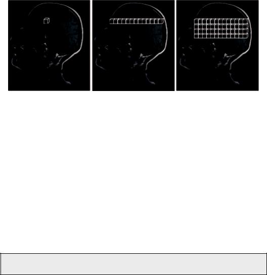
Spectra can be acquired either with a single voxel (SV) technique (single voxel spectroscopy, SVS) or multiple voxel technique, known as either magnetic resonance spectroscopic imaging (MRSI) or chemical shift imaging (CSI) in two (2D CSI) or three dimensions (3D CSI). Of course, the more voxels (2D) or slices (3D), the more time is needed for the acquisition, and the greater the possibility for subject movement. Figure 5.3 schematically illustrates the three MRS techniques.
96 |
Advanced MR Neuroimaging: From Theory to Clinical Practice |
SVS |
2D CSI |
3D CSI |
FIGURE 5.3 Spectra can be acquired either with a single voxel technique (single voxel spectroscopy, SVS) or multiple voxel technique, alternatively called chemical shift imaging (CSI), either in 2D or 3D.
SVS is based on the point resolved spectroscopy (PRESS) (Bottomley and Park, 1984) or the stimulated echo acquisition mode (STEAM) (Frahm et al., 1989) pulse sequences while MRSI uses a variety of pulse sequences (Spin Echo, PRESS, etc.) (Brown et al., 1982; Duyn and Moonen, 1994; Luyten et al., 1990).
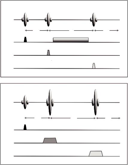
PRESS uses a 90° and two 180° RF pulses in a fashion similar to a standard multi-echo sequence (Figure 5.4b). Each RF pulse is applied using a different physical gradient as the slice selection gradient. Only protons located at the point where all three pulses intersect produce the spin echo at the desired TE.
STEAM uses three selective 90° pulses, each with a gradient on one of the three axes as shown in Figure 5.4a, and is designed to collect only the stimulated echo signal from the area (voxel) of the intersection of all three slices. STEAM has been used for many studies because for many years it was the only sequence capable of short echo times (~30 ms) (Bottomley and Park, 1984; Frahm et al., 1989).
Inevitably the question arises: Which pulse sequence should be used?
The answer is that although there are differences between the two, these are rather subtle and that in practice this mainly depends on the particular availability from the scanner vendor. Nevertheless, there has been a detailed comparison from Moonen et al. (1989) who concluded that the major difference is in the nature of the echo signal. In PRESS, the entire net magnetization from the voxel is refocused to produce the echo signal, whereas in STEAM, a maximum of one-half of the entire net magnetization generates the stimulated echo. As a result, PRESS has a SNR significantly larger than for STEAM for equivalent scan parameters. Another difference is that the voxel dimensions with PRESS may be limited by the high transmitter power for the 180° RF pulses. Finally, and more importantly, STEAM allows for shorter TE values, reducing signal losses from T2 relaxation and allowing observation of metabolites with short T2*.
Although SVS is very useful in clinical practice for several reasons (widely available, short scan times, short TE contains signals from more compounds, etc.), its main disadvantage is that it does not address spatial heterogeneity of spectral patterns and in the context of brain
Magnetic Resonance Spectroscopy |
|
|
97 |
90° |
90° |
90° |
STEAM |
|
|||
RF |
|
|
|
TE/2 |
|
TM |
TE/2 |
Gx |
|
|
|
Gy |
|
|
|
Gz |
|
|
|
|
|
(a) |
|
90° |
180° |
180° |
PRESS |
RF |
|
|
|
TE/4 |
|
TE/2 |
TE/4 |
Gx |
|
|
|
Gy |
|
|
|
Gz |
|
|
|
(b)
FIGURE 5.4 Simplified diagrams of the single voxel pulse sequences. (a) the STEAM sequence and
(b) the PRESS sequence.
tumors. These factors are particularly important, especially for treatment planning in case of radiation or surgical resection.
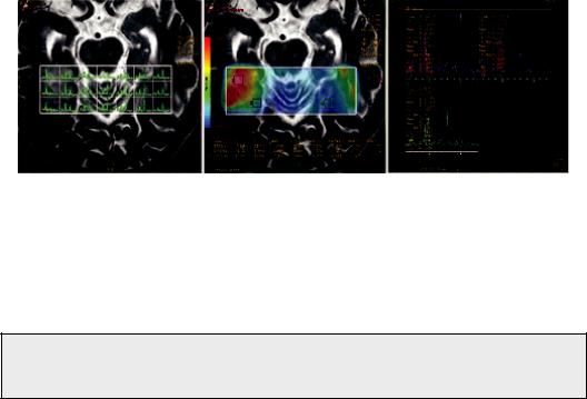
Hence, a lesion’s heterogeneity is better assessed by MRSI. MRSI techniques have been extended to two dimensions (2D) by using phase-encoding gradients in two directions (Duyn et al., 1993; Luyten et al., 1990), or, subsequently, three-dimensional (3D) encoding (Gruber et al., 2003; Nelson et al., 1999). Thus, MRSI techniques allow the detection of localized 1H-MR spectra from a multidimensional array of locations (see Figure 5.5). While technically more challenging due to (1) possibility for significant magnetic field inhomogeneity across the entire volume of interest, (2) the so called “voxel bleeding,” which is a spectral degradation due to intervoxel contamination, (3) longer data acquisition times and (4) challenging post-processing of large
98 |
Advanced MR Neuroimaging: From Theory to Clinical Practice |
FIGURE 5.5 Example of a 2D-MRSI of a patient with a glioma. Left: The lesion on a T2 weighted image. Middle: MRSI data presented as a metabolic map of Choline/Creatine with voxels from multiple locations at the same plane of the lesion. Right: Multiple spectra with metabolite ratios.
multidimensional datasets, MRSI can detect metabolic profiles from multiple spatial positions, thereby offering an unbiased characterization of the entire object under investigation.
Again, inevitably the question arises: Which one should be used in clinical practice, SVS, CSI, or both?
This is not an easy answer. Usually, SVS is performed at short TEs (35 ms) while MRSI at long TEs (135–144 ms). As already mentioned, short TE spectra contain signals from more compounds and have better SNRs; however, they have worse water and lipid contamination when compared to long TEs. On the other hand, long TE spectra have lower SNR and fewer detectable compounds, but they are better resolved with flatter baselines and contain more information in considerably less time. Moreover, MRSI can produce metabolic maps and therefore it can reveal abnormalities in multiple locations. Consequently, the method of choice depends on the clinical information required as well as the position of the area under investigation. If for example a lesion is very close to areas with high magnetic susceptibility (e.g., the sinuses) then MRSI may be impossible to acquire. On the other hand, if spectroscopy is being used to evaluate a disease that is diffuse or covers a large area of anatomy, then spectra from several volumes of tissue can be measured simultaneously, which is advantageous and time saving. Not infrequently, or maybe rather most commonly, a combination of both techniques proves to be the best solution.
5.2.3 Field Strength (B0)
From the very beginning of MRI, optimum field strength was a topic of debate. Nevertheless, for MRS applications the substantial benefit from a high magnetic field was already known for a long time in ex vivo NMR and animal studies. In contrast to MRI, in 1H-MRS clinical applications, a magnetic field of sufficient strength is preferable as it is not the signals of water and fat that are of interest, but rather the considerably smaller metabolites’ signals (about four orders of magnitude). Therefore, most clinical 1H-MRS measurements are performed using MR systems with field strengths of >1.5T. As we all know now, the brilliance of high-field strengths and especially 3T won the race, although even more powerful (4T, 7T, and even higher) body scanners are currently in use.
Magnetic Resonance Spectroscopy |
99 |
3.0T
1.5T
100 200 300 400 500 600 Frequency (Hz)
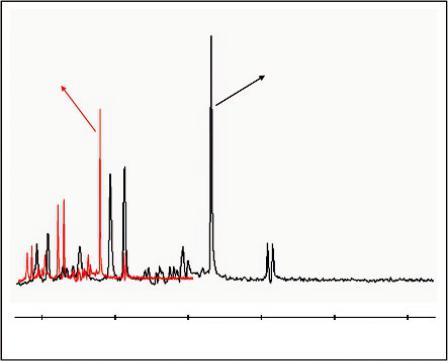
FIGURE 5.6 Comparison of single voxel spectra obtained at 1.5T and 3T, using the protocol (PROBE-P), a standard spectroscopy phantom (25-cm-diameter MRS HD sphere; General Electric Company) and the software provided by the manufacturer (General Electric Medical Systems, Milwaukee, WI). At 3T, the signal-to-noise ratio (SNR) is about 25% higher and the spectral distance between the metabolites (in Hertz) is doubled.
Obviously, the main advantage of increasing the magnetic field strength is the subsequent increase of the signal-to-noise ratio (SNR) since the intensity of the MR signal is correlated linearly with the strength of the static magnetic field. Thus, theoretically, the signal-to-noise ratio (SNR) would double when doubling the field strength (e.g., from 1.5T to 3T); however, when put into clinical practice, the improvement ranges only from 20% to 50%. This is very well illustrated in Figure 5.6 where the overlapping of spectra indicatively emphasizes the differences between 1.5T and 3.0T. It is shown that at 3T, the SNR is about 25% higher and the spectral distance between the metabolites (in Hertz) is approximately doubled.
In the study by Barker et al. (2001), a 28% increase in SNR at 3T compared to that of 1.5T at short TEs was demonstrated, appreciably less than the theoretical 100% improvement. The limited SNR improvement can be explained by several factors including T1 and T2 relaxation, coil and system losses, and RF penetration effects, which strongly affect the linearity between SNR and field strength, as well as type of sequence, number of signal averages and size of sample volume (Di Costanzo et al., 2007; Edelstein et al., 1986; Ocali et al., 1998). Nevertheless, by using particular methods of data acquisition, processing and fitting, SNR can increase by about 80% at 4T compared with that at 1.5T (Bartha et al., 2000) and approximately 100% at 7T compared with 4 T (Tkác et al., 2001). One of the possible approaches to increase the SNR is the use of multiple receiver coils. In fact, a well-designed phased array (PA) head coil has significantly superior sensitivity to that of the birdcagetype volume coil, which is more widely used (De Zwart et al., 2004).
100 |
Advanced MR Neuroimaging: From Theory to Clinical Practice |
Another advantage of the higher magnetic field, is the proportional increase of the Chemical Shift, from 220 Hz at 1.5T to 440 Hz at 3T (Alvarez-Linera, 2008). Consequently, this is reflected by a more effective water suppression and improved baseline separation of J-coupled metabolites, without the need of sophisticated spectral editing techniques (Barker et al., 2001; Bartha et al., 2000; Stephenson et al., 2011). The improvement in spectral resolution is more evident at 7T where weakly represented neurochemicals with important clinical impact, such as scylloIns, aspartate, taurine and NAAG, can be clearly estimated (Stephenson et al., 2011; Tkác et al., 2001).
5.2.4 Voxel Size Dependency
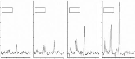
At lower field strengths (≤1.5 T) the suggested minimum voxel size is 2 × 2 × 2 cm (i.e., 8 cm3). At higher field strengths (≥3 T) most 1H-MRS studies have been performed with a minimum spatial resolution of 1 cm3 (Gruber et al., 2003). Figure 5.7 depicts the dependency of SNR to the voxel size. It is evident that increasing the voxel sizes increases the SNR while the acquisition time remains constant.
Reducing voxel’s size substantially reduces the SNR since these two are linearly proportional. Nevertheless, at fields of 3T or higher, voxels below 1 cm3 can be obtained with acceptable SNR (Boer et al., 2011; Gruber et al., 2003), but with rather long acquisition times (see also Section 6.2.4). Hence, reduced voxel sizes can improve the sensitivity and specificity of diagnosis and enable the creation of metabolic maps that depict details of heterogeneous lesions such as gliomas, where changes in their development can occur in small areas. Nevertheless, intrinsic field-dependent technical difficulties may affect the aforementioned advantages and should be considered. When the frequency shift between two adjacent nuclei is large enough, a measurable alteration of the MR signal, used to encode the x- and y-axis spatial coordinates, will occur producing a spatial misregistration. This means that the volume of MRS information may not be the same as that displayed on the localizer MR image (Di Costanzo et al., 2003). More importantly, in high magnetic field strengths, magnetic susceptibility from paramagnetic substances and blood products are sensibly increased (Gu et al., 2002). Consequently, magnetic field inhomogeneity and susceptibility artifacts complicate the extraction of good-quality spectra, especially from largely heterogeneous lesions
30 |
30 |
|
|
|
|
|
|
30 |
|
|
30 |
|
|
|
|
1 cm3 |
2 cm3 |
|
|
|
|
|
4 cm3 |
|
8 cm3 |
|
|
||
25 |
25 |
|
|
|
|
|
|
25 |
|
|
25 |
|
|
|
20 |
20 |
|
|
|
|
|
|
20 |
|
|
20 |
|
|
|
15 |
15 |
|
|
|
|
|
|
15 |
|
|
15 |
|
|
|
10 |
10 |
|
|
|
|
|
|
10 |
|
|
10 |
|
|
|
5 |
5 |
|
|
|
|
|
|
5 |
|
|
5 |
|
|
|
0 |
0 |
|
|
|
|
|
|
0 |
|
|
0 |
|
|
|
|
4.0 3.5 3.0 2.5 2.0 1.5 1.0 0.5 0.0 |
4.0 |
3.5 |
3.0 |
2.5 |
2.0 |
1.5 |
1.0 |
4.0 3.5 |
3.0 2.5 2.0 |
1.5 1.0 0.5 0.0 |
4.0 3.5 3.0 2.5 |
2.0 1.5 1.0 0.5 |
0.0 |
FIGURE 5.7 Dependency of SNR to the voxel size. Spatial resolution of 1 cm3 is practically considered a minimum.
Magnetic Resonance Spectroscopy |
101 |
(Di Costanzo et al., 2003). Nevertheless, improvement of the local shimming methods can alleviate the problem (see next section).
5.2.5 Shimming
Shimming refers to the process of adjusting the field gradients of the scanner system in order to optimize the magnetic field homogeneity over the volume under study.
In case you are wondering (as I did), the word shimming originates from the thin sheets of iron that were originally used by engineers to adjust the uniformity of magnets called “shims.” Magnetic field inhomogeneities result primarily from susceptibility differences between different tissues and between tissue and air cavities, which are scaled non-linearly in ultra-high magnetic fields (Avdievich et al., 2009). Thus, voxels that are placed in, or near inhomogeneous regions of the brain, such as the temporal poles, are difficult to shim due to their close proximity to the sinuses.
In any case it has to be stressed here that there is no such thing as a perfectly homogeneous magnetic field because it cannot be produced, and even if it could, the insertion of the patient into the scanner would immediately make it imperfect due to the so-called susceptibility effects. These effects are produced by inhomogeneities such as the aforementioned air-filled areas (sinuses or intestines) or dense bone (skull base), which change the main magnetic field in their immediate vicinity, so tissues around such inhomogeneities will experience different magnetic fields.
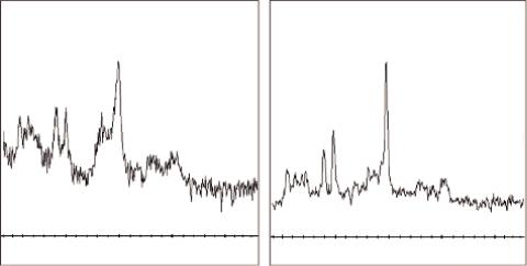
Hence, field homogeneity is specified by measuring the full width at half maximum (FWHM) of the water resonance, which determines the spectral resolution. Special emphasis must be given to shimming, especially in high field strengths, as it increases both sensitivity and spectral resolution. This is why most devices come equipped with second or third order shimming (Avdievich et al., 2009) by monitoring either the time domain or frequency domain of the 1H-MRS signal (Drost et al., 2002). Especially in cases when field homogeneity should be reached in large volumes of interest, as in the case of MRSI, 4-order shimming might be necessary (Hetherington et al., 2006; Gillard et al., 2010. Figure 5.8 illustrates the difference between a good shimming and a bad shimming procedure.
|
NAA |
|
NAA |
Cho Cr |
Glx |
|
|
|
|
|
|
ml |
|
Cr |
|
|
Lipids + Lactate |
Cho |
Glx |
|
|
ml |
|
|
|
Lipids + Lactate |
|
|
|
|
4 |
3 |
2 |
1 |
0 |
4 |
3 |
2 |
1 |
0 |
|
|
|
|
WW:400 WL:200 |
|
|
|
|
WW:400 WL:200 |
|
|
|
(a) |
|
|
|
|
(b) |
|
FIGURE 5.8 Notice the difference between (a) inadequate shimming (linewidth = 13 Hz) and (b) adequate shimming (linewidth = 5 Hz).
102 |
Advanced MR Neuroimaging: From Theory to Clinical Practice |
A minimum of 6 Hz at 1.5T and 10 Hz at 3.0T linewidth is considered to be an adequate shimming for SVS, taking into account that 0.1 ppm equals approximately to 6 Hz at 1.5T. Shimming can be performed either manually or automatically. Manual shimming requires a great deal of expertise and therefore, in a well-maintained scanner, automatic shimming is considered a safer and more reproducible option.
Effective shimming requires methods for mapping a field’s strength variations over the area under study. Methods that have been developed for field mapping can be grouped into two categories: those based on 3D field mapping (Hetherington et al., 2006; Miyasaka et al., 2006) and those that map the magnetic field along projections (Zhang et al., 2009). In both shimming methods, information about the magnetic field variation is calculated from phase differences acquired during the evolution of the magnetization in a non-homogeneous field.
5.2.6 Water and Lipid Suppression Techniques
Water protons are at such a high concentration compared with the other proton containing metabolites, the water peak obviously dominates the spectrum and makes the other peaks impossible to measure. The same applies for lipids, hence water and peri-cranial lipid suppression techniques are of paramount importance in 1H-MRS procedures in order to observe in detail the much less concentrated metabolite signals.
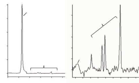
The metabolites of interest are usually several orders of magnitude less in concentration than water. Therefore, the water suppression efficiency should be robust and should not vary spatially across the field of view (FOV). This is illustrated in Figure 5.9.
The existing water suppression techniques can be divided into three major groups, namely:
(1) methods that employ frequency-selective excitation and/or refocusing pulses; or (2) utilize differences in relaxation parameters; and (3) other methods, including software-based water suppression.
The most common method of the first group utilizes multiple (typically three) frequencyselective 90° pulses (chemical shift selective water suppression (CHESS) pulses (Haase et al., 1985), prior to localization pulse sequence. Additionally, suppression can be achieved
1000
H2O
25
800 |
|
|
|
|
|
|
|
Metabolites |
|
|
|
|
||
|
|
|
|
|
|
|
|
|
|
|
|
|||
|
|
|
|
|
20 |
|
|
|
|
|
|
|
|
|
600 |
|
|
|
|
|
|
|
|
|
|
|
|
|
|
|
|
|
|
|
15 |
|
|
|
|
|
|
|
|
|
400 |
|
|
|
|
10 |
|
|
|
|
|
|
|
|
|
|
|
|
|
|
|
|
|
|
|
|
|
|
|
|
200 |
|
|
|
|
5 |
|
H2O |
|
|
|
|
|
|
|
|
|
Metabolites |
|
|
|
|
|
|
|
|
|
|
||
|
|
|
|
|
|
|
|
|
|
|
|
|
||
|
ppm |
|
|
|
0 |
ppm |
|
|
|
|
|
|
|
|
0 |
|
|
|
|
|
|
|
|
|
|
|
|||
|
|
|
|
|
|
|
|
|
|
|
|
|||
|
|
|
|
|
|
|
|
|
|
|
|
|
|
|
6 |
5 |
4 |
3 |
2 |
1 |
5.0 |
4.5 |
4.0 |
3.5 |
3.0 |
2.5 |
2.0 |
1.5 |
1.0 |
FIGURE 5.9 Left: Before water suppression, the metabolite peaks under investigation are depicted as noise. Right: After water suppression, the metabolites are revealed.
Magnetic Resonance Spectroscopy |
103 |
by selectively diphase water, while metabolites of interest are rephased using refocusing pulses during the spin-echo period. The three spin-echo-based methods are WATERGATE (Piotto et al., 1992), excitation sculpting (Hwang and Shaka, 1995) and MEGA (Mescher et al., 1996).
As water and metabolite T1s are sufficiently different, it is possible to suppress the water signal and observe the metabolites in the close proximity to the water resonance. WEFT (water eliminated Fourier transform) is among the oldest T1-based water suppression methods (Patt and Sykes, 1972), which is identical to an inversion recovery sequence used for T1 relaxation time measurements. Water suppression can be further optimized by applying a band-selective inversion with a gradient dephasing pulse (BASING), alone or with addition of CHESS (Star-Lack et al., 1997).
The third method includes two separate scans with metabolite resonances inversion. The water resonance is not inverted in either scan. Therefore, the difference between the first and second scan will result in the subtraction of water and hence water suppressed metabolite spectrum.
Lipid suppression can be performed by avoiding the excitation of the lipid signal using STEAM or PRESS localization, hence suppressing their contribution to the detected signal.
Opposite to the strategy employed by volume pre-localization, outer volume suppression pulses (OVS) are applied to pre-saturate the lipid signal (Duyn et al., 1993). As illustrated in Figure 5.10, rather than avoiding the spatial selection of lipids, OVS excites narrow slices of the brain’s lipid-rich regions.
FIGURE 5.10 Upper part: The location and orientation of OVS pulses have been prescribed in order to saturate as much peri-cranial lipid as possible while the signal within the voxel remains unperturbed. Lower part, left: The application of two extra saturation bands. Lower part, right: The two extra bands with the default bands are illustrated.
104 |
Advanced MR Neuroimaging: From Theory to Clinical Practice |
Additionally, the difference in T1s of lipids (250–350 ms) and metabolites (1000–2000 ms) allow the application of an inversion pulse (inversion time ~200 ms), which will selectively null the lipid signal (Spielman et al., 1992). If the inversion delay is appropriately chosen, the longitudinal lipid magnetization will be zero, so the lipids will be nulled. The aforementioned suppression methods are usually better implemented in long TE spectra as both water and lipid resonances have shorter T2 relaxation times than many metabolites.
At this point it is very important to stress that MRS sequences apply a number of presaturation bands by default (left-right, posterior-anterior, superior-inferior) as illustrated in Figure 5.10, lower right. The addition of extra saturation bands is possible but there is always a limit (usually 10, i.e., +4). After this limit, the extra bands gradually delete default saturation bands with an unknown order and this has to be taken into account!
5.3 MRS Metabolites and Their Biological and Clinical
Significance
Focus Point
•Metabolite ratios provide robust in vivo markers of biochemistry but they should be interpreted with caution.
•N-acetyl-aspartate: Detected in neuronal and non-neuronal cells. Considered as a neuron’s integrity index.
•Total choline: Metabolic index of membrane density and integrity.
•Total creatine: Present in both neuronal and glial cells. Serves as an energy buffer and energy shuttle. Can be used as the reference metabolite.
•Myo-inositol: Glial and myelin degradation marker. Malignant tumor indicator.
•Lactate: Present in both intracellular and extracellular spaces. Product of anaerobic glycolysis. Increases in tumors.
•Lipids: Membrane breakdown and necrosis index. Increases in high grade tumors.
•Glx complex (Glu/Gln): Provides detoxification and regulation of neurotransmitters. Difficult to separate complex’s peaks.
The aim of in-vivo 1H-MRS is to use metabolite levels for an accurate evaluation of cerebral lesions, and therefore, determination of the relationship between metabolic profile and pathologic processes is required. The biological and clinical significance of the basic resonances in a spectrum, as well as the less commonly detected ones, is discussed in this section. For a more comprehensive overview of the assignment and significant role of each brain metabolite evaluated, a summary is depicted in Table 5.1. The light shade represents difficulty in separating low filed strengths, and the darker shade represents the metabolites that are elevated/detected only in pathological conditions. Basic resonances detected in the normal brain are not shaded.
5.3.1 Myo-Inositol
Starting from left to right of the indicative spectrum of Figure 5.2a, Myo-inositol (mI–3.56 ppm) is a cyclic sugar alcohol that gives rise to four groups of resonances with the

Magnetic Resonance Spectroscopy |
|
105 |
||
TABLE 5.1 List of Metabolites Detected in the Human Brain by Proton MR Spectroscopy |
||||
|
|
|
|
|
Metabolite |
Chemical Shift |
Physiological Significance |
Increased |
Decreased |
|
|
|
|
|
NAA |
2.02 ppm |
Healthy neuronal cell |
Very rarely |
Commonly: |
(N-acetyl |
|
marker. |
Canavan’s disease |
nonspecific |
aspartate, other |
|
Only seen in nervous |
|
neuronal loss or |
N-acetyl |
|
tissue. |
|
dysfunction due to |
moieties) |
|
Exact physiological role |
|
range of insults, |
|
|
uncertain. |
|
including |
|
|
|
|
ischemia, trauma, |
|
|
|
|
gliosis |
|
|
|
|
inflammation, |
|
|
|
|
infection, tumors, |
|
|
|
|
dementia, |
Cho |
3.2 ppm |
Detectable resonance is |
Tumors, |
Stroke, |
Choline |
|
predominantly choline |
inflammation, |
encephalopathy |
containing |
|
derivatives. Marker of |
chronic hypoxia |
(hepatic human |
compounds |
|
membrane turnover. |
|
immunodeficiency |
|
|
Higher in WM than GM. |
|
virus (HIV)/liver |
|
|
Increase with age. |
|
disease |
Cr |
3.0 ppm |
Compounds related to |
Trauma, |
Hypoxia, stroke, |
Creatine/ |
|
energy storage; thought |
hyperosmolar states |
tumors |
Phospho-creatine |
|
to be marker of energetic |
|
|
|
|
status of cells. Other |
|
|
|
|
metabolites are |
|
|
|
|
frequently expressed as |
|
|
|
|
ratio to Cr. Low in |
|
|
|
|
infants. |
|
|
|
|
Increases with age. |
|
|
mI(Myo) |
3.56 ppm (short |
Pentose sugar, osmolyte, |
Neonates, |
Malignant tumors, |
Myo-inositol |
TE only) |
glial cell marker. High in |
Alzheimer’s, |
chronic hepatic |
(other inositols) |
|
infants. |
diabetes, low-grade |
encephalopathy, |
|
|
|
glioma recovered |
stroke |
|
|
|
encephalopathy, |
|
|
|
|
hyperosmolar states |
|
Glx |
2.1–2.4 ppm |
Complex overlapping |
Hepatic |
Possibly |
Glutamate (Glu) + |
(short TE |
J–coupled resonances |
encephalopathy, |
Alzheimer’s |
Glutamine (Gln) |
only) |
difficult to separate and |
severe hypoxia, |
disease |
|
|
quantify at clinical field |
OTC deficiency |
|
|
|
strengths (1.5–3T). |
|
|
|
|
Amino acid |
|
|
|
|
neurotransmitters Glu |
|
|
|
|
excitatory, Gln inhibitory. |
|
|
Lactate |
1.35 ppm |
Not seen in normal adult |
Ischemia, inborn |
- |
|
(doublet, 7 |
brain. End product of |
errors of metabolism |
|
|
ppm |
anaerobic respiration. |
tumors (all grades), |
|
|
separation) |
Thought to be elevated |
abscesses, |
|
|
|
in foamymacrophages. |
inflammation |
|
Lipids |
0.9 and 1.3 ppm |
Not seen in normal brain. |
High-grade tumors, |
- |
Mobile lipid |
(short TE |
Membrane breakdown/ |
abscesses, acute |
|
moieties |
unless ↑↑) |
lipid droplet formation. |
inflammation, |
|
|
|
May precede histological |
acute stroke |
|
|
|
necrosis. |
|
|
(Continued)

106 Advanced MR Neuroimaging: From Theory to Clinical Practice
TABLE 5.1 (Continued) List of Metabolites Detected in the Human Brain by Proton MR Spectroscopy
Metabolite |
Chemical Shift |
Physiological Significance |
Increased |
Decreased |
|
|
|
|
|
Alanine |
1.47 ppm |
Amino acid present in the |
Meningiomas (?) |
|
|
|
normal brain. |
|
|
Succinate, acetate, |
2.4 ppm, 1.92 |
Products of bacterial |
Pyogenic abscesses |
- |
amino acids |
ppm, 0.9 ppm |
metabolism. |
|
|
Acetoacetate, |
Not normally |
Only pathologically |
Inborn errors of |
- |
acetone |
detectable |
elevated in inborn |
metabolism |
|
|
|
errors. |
|
|
Mannitol, ethanol |
Various |
Administered drugs and |
|
- |
|
|
other substances. |
|
|
larger and most important signal occurring at 3.56 ppm. It is observable on short time echo (TE) spectra as it exhibits short T2 relaxation times and is susceptible to dephasing effects due to J-coupling.
Interestingly, the exact function of mI is still uncertain (Ross, 1991), however it has been proposed as a glial marker (Brand et al., 1993) and an increase of mI levels is believed to represent glial proliferation or an increase in glial cell size, both of which may occur in inflammation (Soares and Law, 2009). Additionally, this metabolite is involved in the activation of protein C kinase, which leads to production of proteolytic enzymes found in malignant and aggressive cerebral tumors, serving as a possible index for glioma grading (Castillo et al., 2000). mI has also been labeled as a breakdown product of myelin (Kruse et al., 1993) since altered levels of mI have been encountered in patients with degenerative and demyelinating diseases (Lin et al., 2005; Wang et al., 2009; Wattjes and Barkhof, 2008; Wattjes et al., 2009).
5.3.2 Choline-Containing Compounds
Choline-containing compounds (tCho–3.22 ppm) comprise signals from free choline (Cho), phosphocholine (PC) and glycerophosphocholine (GPC), with a resonant peak located at 3.22 ppm. Since the resonance contains contributions from several methyl proton choline-contain- ing compounds, it is often referred as “total Choline” (tCho).
tCho is involved in pathways of phospholipid synthesis and degradation, thus reflecting a metabolic index of membrane density and integrity as well as membrane turnover (Howe et al., 2003; Möller-Hartmann et al., 2002; Nelson et al., 1999; Sibtain et al., 2007; Soares and Law, 2009).
Consistent changes of tCho signals have been observed in a large number of cerebral diseases. Processes that lead to elevation of tCho include accelerated membrane synthesis of rapidly dividing cancer cells in brain tumors (Howe et al., 2003; Sibtain et al., 2007; Kararizou et al., 2006; Soares and Law, 2009), cerebral infractions, infectious diseases (Calli et al., 2002; Lai et al., 2008), and inflammatory-demyelinating diseases (Hayashi et al., 2003; Malhotra et al., 2009).
It has to be stressed that tCho exhibits a physiologic marked regional variability with higher concentrations observed in the pons and lower levels in the vermis and dentate (Mascalchi et al., 2002). Detailed knowledge about regional variations of tCho is necessary for an accurate interpretation of tCho levels, especially in diseases such as epilepsy and psychiatric disorders where tCho levels are subtly different to normal levels.
Magnetic Resonance Spectroscopy |
107 |
5.3.3 Creatine and Phosphocreatine
Creatine and Phosphocreatine (tCr–3.03 ppm and 3.93 ppm) together are often referred as total creatine (tCr) because they cannot be distinguished with a standard clinical MR unit (up to 7T) and their sum is thus mentioned. Cr and PCr arise from the methyl and methylene protons of Cr and phosphorylated Cr. tCr is located at 3.03 ppm and 3.93 ppm resonant frequencies.
In the brain tCr is present in both neuronal and glial cells and is involved in energy metabolism serving as an energy buffer via the creatine kinase reaction retaining constant ATP levels; it also serves as an energy shuttle, diffusing from mitochondria to the nerve terminals in the brain. (De Graaf, 2007). As tCr is not naturally produced in the brain, its concentration is assumed to be stable with no changes reported with age or a variety of diseases, and is used as a reference value for calculating metabolite ratios (e.g., NAA/Cr, tCho/Cr, etc.). Nevertheless, the use of tCr as a reference metabolite should be used with caution as decreased tCr levels have been observed in the chronic phases of many pathologies including tumors (Howe et al., 2003; Ishimaru et al., 2001), stroke (Gideon et al., 1992), and gliosis (van der Graaf, 2010).
5.3.4 Glutamate and Glutamine
Glutamate (Glu–2.15 ppm) and Glutamine (Gln–2.45 ppm) together form a complex of peaks (Glx complex) between 2.15 ppm and 2.45 ppm. Their distinction at 1.5T is difficult due to their similar chemical structures. However, at ≥3T Glu and Gln can be resolved (Srinivasan et al., 2006) and at magnetic fields of 7T and higher, the Glu and Gln resonances are visually separated, leading to considerable quantification accuracy (De Graaf, 2007).
Glu is the major excitatory neurotransmitter in the mammalian brain and the direct precursor for the major inhibitory neurotransmitter, γ-aminobutyric acid (GABA). Besides these roles, Glu is also an important component in the synthesis of other small metabolites (e.g., Glutathione) as well as larger peptides and proteins. The amino acid Gln, which is primarily located in astroglia, is involved in intermediary metabolism and is synthesized from Glu (De Graaf, 2007). The Glx complex plays a role in detoxification and regulation of neurotransmitters. Increased levels of Glx complex are markers of epileptogenic processes (Hammen et al., 2003; Simister et al., 2009) and decreased levels of Glx have been observed in Alzheimer, dementia and patients with chronic schizophrenia (Kantarci et al., 2003; Théberge et al., 2003). Glx complex increments have also been observed in the peritumoral brain edema correlated with neuronal loss and demyelination (Ricci et al., 2007). As reported by Srinivasan et al. (2005), Glx might be used as an in vivo index of inflammation since they observed elevated Glx levels in acute MS plaques but not in chronic ones.
5.3.5 N-Acetyl Aspartate
N-Acetyl Aspartate (NAA–2.02 ppm) in 1H-MR spectra of normal brain, is the most prominent resonance originating from the methyl group of NAA at 2.02 ppm with a contribution from neurotransmitter N-aspartyl-glutamate (NAAG) (Frahm et al., 1991). NAA is exclusively localized in the central and peripheral nervous system synthesized in brain mitochondria. Its concentration varies subtly in different parts of the brain (Baker et al., 2008; Doelken et al., 2009; Pouwels and Frahm, 1998) but undergoes large developmental changes, almost doubling from birth to adulthood (Kreis et al., 1992; Toft et al., 1994; Barker, 2001). Although NAA is definitely considered a neuronal marker representing neuronal density and viability, its exact function remains largely unknown. Possible neuronal functions of NAA include osmoregulation (Taylor et al., 1995) and a breakdown product of NAAG (Blakely and Coyle, 1988; Martin et al., 2001).
108 |
Advanced MR Neuroimaging: From Theory to Clinical Practice |
The utility of NAA as an axonal marker is supported by the loss of NAA in many white matter diseases, including leukodystrophies (Morita et al., 2006; Távora et al., 2007), multiple sclerosis (MS) (Mader et al., 2008; Wattjes et al., 2008) and hypoxic encephalopathy (Rosen and Lenkinski, 2007), chronic stages of stoke (Mader et al., 2008; Saunders, 2000) and tumors (Howe et al., 2003; Law et al., 2002; Nelson et al., 2003; Sibtain et al., 2007; Soares and Law, 2009).
However, there are cases when the abnormal levels of NAA do not reflect changes in neuronal density, but rather a perturbation of the synthetic and degradation pathways of the NAA metabolism. For instance, in Canavan’s disease, high levels of intracellular NAA (Barker et al., 1992; Lin et al., 2005) are due to deficiency of aspartoacylase (ASPA), which is the enzyme that degrades NAA to acetate and aspartate. Further examples that show the lack of direct relationship of NAA to neuronal integrity include various pathologies such as temporal lobe epilepsy (TLE) (Chernov et al., 2009; Hajek et al., 2008; Lee et al., 2005) or amyotrophic lateral sclerosis (ALS) (Sarchielli et al., 2001; Wang et al., 2006), which exhibit spontaneous or treatment reversals of NAA to normal levels (Barker et al., 2001).
NAA has been also detected in non-neuronal cells, such as oligodendrocytes, which may contribute to the overall NAA signal observed in a 1H-MRS spectrum, suggesting that it may not be specific only for neuronal processes (Bhakoo and Pearce, 2000).
5.3.6 Lactate and Lipids
Lactate and free Lipids (Lac–1.35 ppm, Lip–0.9–1.3 ppm), should be maintained below or at the limit of detectability within the normal brain spectrum, overlapping with macromolecule (MM) resonances at 1.33 ppm (doublet) and 0.9–1.3 ppm, respectively. Any detectable increase of lactate and lipid resonances can therefore be considered abnormal.
Lac is present in both intracellular and extracellular spaces and can be considered an index of metabolic rate being the end-product of anaerobic glycolysis (Howe et al., 2003). Hence, increased lactate levels can been observed in a wide variety of conditions in which oxygen supply is restricted, such as acute and chronic ischemia (Graham et al., 1992; Mader et al., 2008; Saunders, 2000), metabolic disorders (Chi et al., 2011; Soares and Law, 2009; Cecil, 2006), and tumors (De Graaf, 2007; Howe et al., 2003; Nelson et al., 2003; Sibtain et al., 2007; Soares and Law, 2009).
Lactate also accumulates in tissues that have poor washout, like cysts (Chang et al., 1998; Mishra et al., 2004) and normal pressure hydrocephalus (Kizu et al., 2001). The aforementioned spectral region between 0.9 ppm and 1.3 ppm represents the methylene (1.3 ppm) and the methyl (0.9 ppm) groups of fatty acids. Fractured proteins and lipid layers become visible only during the breakdown of membranes. Regardless of the exact mechanism, an elevation of lipid resonances indicates cerebral tissue destruction such as infarction (Graham et al., 1992; Mader et al., 2008; Saunders, 2000), acute inflammation (Hayashi et al., 2003; Yeh et al., 2008), and necrosis (Ishimaru et al., 2001; Lai et al., 2008).
5.3.7 Less Commonly Detected Metabolites
The signals of most other metabolites in a brain spectrum are considerably smaller than those mentioned so far, often due to their splitting into multiplets and/or overlapping peaks. Some of these compounds are present in healthy brain tissue but because they are too small, their detection is difficult. Some examples of these compounds include Alanine, Glycine, Taurine, Glutathione, and several other amino acids such as Succinate, Acetate, Valine and Leucine.
Magnetic Resonance Spectroscopy |
109 |
Alanine (Ala–1.47 ppm) is an amino acid present in the normal brain, resonating at 1.47 ppm. It is frequently considered a specific metabolic characteristic of meningiomas, however, its identification rate varies from 32% to 100% (Bulakbasi et al., 2003; Chernov et al., 2011; Cho et al., 2003; Demir et al., 2006; Howe et al., 2003; Möller-Hartmann et al., 2002). It can also be present in neurocytomas (Krishnamoorthy et al., 2007), gliomas (Majós et al., 2004), and PNETs (Majós et al., 2002). In vivo 1H-MRS at lower filed strengths often cannot provide a distinction between Ala and Lac peaks as they resonate in neighboring frequencies. When both metabolites are present, they produce a triplet peak located between 1.3 ppm and 1.5 ppm (Yue et al., 2008) observed at 3T and higher.
Glycine (Gly–3.55 ppm) is considered an inhibitory neurotransmitter (Yeh et al., 2008) and a possible antioxidant, distributed mainly in astrocytes and glycinergic neurons. It resonates at 3.55 ppm, overlapping with mI; therefore, its detection is impossible in a nonprocessed spectrum. Only in cases of mI absence, even low Gly levels can be quantified (Lehnhardt et al., 2005).
High levels of Gly have been observed in glioblastomas, medulloblastomas, ependymomas (Kinoshita and Yokota, 1997) and neurocytomas (Yeh et al., 2008). Some research groups have reported that this metabolite may provide a noticeable metabolic feature for the distinction of GBMs from lower grade astrocytomas (Kinoshita and Yokota, 1997; Lehnhardt et al., 2005), primary gliomas from recurrence (Lehnhardt et al., 2005) and glial tumors from metastatic brain tumors (Kinoshita and Yokota, 1997; Majós et al., 2003).
Taurine (Tau–3.25 ppm and 3.42 ppm) gives two triplets at 3.25 ppm and 3.42 ppm, significantly overlapping with Cho and mI. Tau is an inhibitory neurotransmitter that activates GABA-a receptors or strychnine-sensitive glycine receptors, and it has also been suggested as an osmoregulator and a neurotransmitter action modulator (Shirayama et al., 2010).
In a healthy brain, Tau is heterogeneously distributed throughout the brain, with the higher levels observed in the olfactory bulb, retina and cerebellum (Huxtable, 1989).
High levels of Tau have been observed in medulloblastoma (Panigrahy et al., 2006), pituitary adenoma and metastatic renal cell carcinoma (Kinoshita and Yokota, 1997). Increased levels of Tau have been also reported in the medial prefrontal cortex in schizophrenic patients (Shirayama et al., 2010).
Glutathione (GSH–2.9 ppm) is the major protective molecule of living cells resonating at 2.9 ppm. It has an important role against oxidative stress, serving as an antioxidant and detoxifier (An et al., 2009), and plays a role in apoptosis and amino acid transport (Opstad et al., 2003). This metabolite has been reported to participate in acute ischemic stroke patients as ischemia is associated with significant oxidative stress (An et al., 2009), and in other neurodegenerative diseases such as Parkinson’s disease (Sian et al., 1994). GSH has also been found to be significantly elevated in meningiomas when compared to other tumors (Kudo et al., 1990; Opstad et al., 2003), showing, as well, an inverse relationship with glioma malignancy (Couldwell et al., 1992; Kudo et al., 1990).
Finally, several other amino Acids such as Succinate at 2.4 ppm, Acetate at 1.92 ppm, Valine and Leucine at 0.9 ppm, together with Alanine and Lactate, are the major spectral findings of bacterial and parasitic diseases. Acetate and Succinate presumably originate from enhanced glycolysis of the bacterial organism (Chang et al., 1998; Sibtain et al., 2007). The amino acids Valine and Leukine are known to be the end-products of proteolysis by enzymes released in pus (Sibtain et al., 2007). Specifically, Leucine and Valine peaks have been detected in cystercercosis lesions but not in spectra of brain tumors (Sibtain et al., 2007).

110 |
Advanced MR Neuroimaging: From Theory to Clinical Practice |
5.4 MRS Quantification and Data Analysis
Focus Point
Quantification:
•Metabolite ratios are considered robust and reproducible in a clinical environment, but are based on the assumption that total Cr remains constant, which might not be the case.
•Possible abnormal metabolite ratios may be the result of changes in both the numerator and denominator.
•Absolute quantification allows detection of metabolite abnormalities that might not be otherwise evaluated.
•Absolute quantification requires internal or external references, and correction for voxel contamination.
•Post processing:
•Several specialized processing steps are necessary to improve the visual appearance of the MR spectrum or the accuracy during metabolites estimation.
5.4.1 Quantification
To produce a high-quality spectrum, the first step is to obtain the maximum signal strength of each metabolite in a given spectrum and determine its concentration. Of course, several specialized processing steps by sophisticated computer algorithms are performed on the acquired FID, either in the time domain or the frequency domain (i.e., before or after the Fourier transform). These processes are usually not seen by the user since they are performed by automated programs (different vendors use different programs), but play a major role on the quality of analyses. Quantitative analyses of the (spectral) data, as well as the methods for this analysis arguably have the same importance as the techniques used to collect them. Possible incorrect data analysis or potential artifacts and pitfalls may lead to systematic errors and hence misinterpretation of the clinical results.
The quantification of spectra is of paramount importance in in-vivo MRS since visual evaluation alone is obviously not enough. In terms of quantification, the “holy grail” of spectral analysis is to determine the concentrations of the compounds present in the human brain and evaluate them accordingly. That is, to determine the area under the spectral peak, which should be proportional to the metabolite concentration. Nevertheless, this process can be very challenging due to several reasons, such as resonance overlap, baseline distortions, and poorly approximated lineshapes with conventional models such as Gaussian or Lorentzian functions.
On the other hand, spectra can be simply quantified in terms of metabolite ratios rather than metabolite concentrations and it is the most common approach. This sounds safer since metabolite ratios are calculated by dividing the area of each metabolite peak by the area of a reference peak (commonly total Cr) from the same spectrum, thus providing a sound value. Consequently, this approach might remove systematic errors and provide reliable markers of tissue biochemistry. Unfortunately, the technique is based on the assumption that total Cr remains constant and this might not always be the case. Total Cr can be vastly modified across diseases or even during normal brain development or aging. Moreover, it is evident that possible abnormal metabolite ratios may be the result of changes in both the numerator and denominator.

Magnetic Resonance Spectroscopy |
111 |
Therefore, absolute metabolite concentrations can be considered better for in vivo spectra interpretation, despite the involved difficulties.
So once again, inevitably the question arises: To quantify or not to quantify?
Unfortunately, there is no easy answer to this question. There are a variety of approaches and each one has its own set of advantages and disadvantages. The final decision ultimately depends on the clinical problem to be addressed, the experimental conditions used to obtain the data, and the analysis software available to the investigator. For a more comprehensive explanation of the quantification techniques and their pros and cons, please refer to the more detailed Chapter 6 (Section 6.2.8).
5.4.2 Post Processing Techniques
Again, in order to produce a high quality spectrum, several specialized processing steps can be performed retrospectively, improving the visual appearance of the MR spectrum or the accuracy during metabolite estimation. Therefore, for a reliable analysis of in vivo 1H-MR spectra, an understanding of the principles of post-processing techniques is essential.
Signal post-processing can be performed either in the time domain or after Fourier transformation in the frequency domain (Tchofo and Baleriaux, 2009). The most common postprocessing techniques for effective signal improvement are: (1) Eddy current correction, (2) removal of unwanted spectral components, (3) signal filtering, (4) zero filling, (5) phase correction, and (6) baseline correction.
Eddy current correction: During signal localization RF pulses are applied together with magnetic field gradients and additional crusher gradients are needed to eliminate the unwanted signal. The switching pattern of the gradients applied can cause eddy current (EC) artifacts that are time and space dependent, causing time dependent phase shifts in the FID and distorted metabolite lineshapes within the spectrum preventing accurate quantification (see also Chapter 2). In a spectrum, EC artifacts can be removed by acquiring an additional FID without water suppression. The phase of the water FID is determined in each time point and it is subtracted from the phase of the corrupted FID (van der Graaf, 2009). Alternative methods for EC correction without the need for an additional reference peak (e.g., water) have also been proposed making the phase-distorted signal in the spectrum resonate at a different frequency than the remaining components, or using the acquisition of two sequences with opposite gradients (Lin et al., 1994). The EC artifact correction comprises the first step of the post-processing procedure.
The removal of unwanted signals from the FID, which may disturb signals from the resonances of interest, is the next step of signal post-processing. The water signal is a typical example of such an unwanted peak. Water suppression during measurement is never perfect and a residual water signal remains in the spectrum, which often has a complicated lineshape (Jiru, 2008; van der Graaf, 2009). Residual water elimination from the FID can be achieved either by approximating the water signal and subtracting it from the FID (Pijnappel et al., 1992), by eliminating it using special filters (Coron et al., 2001; Sundin et al., 1999), or by applying baseline correction for the removal of the broad water peak from the spectrum (Jiru, 2008).
Quantitative analysis may be hampered by the existence of a distorted spectral baseline as the estimation of metabolite peak areas is not reliable. The baseline signal mostly comprises fast

112 |
Advanced MR Neuroimaging: From Theory to Clinical Practice |
decaying components with very short T2* values such as macromolecules, the signal from the sample and residuals from inefficient water suppression. Therefore, baseline correction is crucial for robust data evaluation and quantification methods. Delayed acquisition (e.g., TE > 80 ms) can remove the macromolecules due to their shorter T2 relaxation times ( 30 ms). But this has a significant drawback, namely the loss of information of many scalar-coupled resonances, which have been suggested to provide valuable information regarding tumor characterization (Castillo et al., 2000; Howe et al., 2003; Ricci et al., 2007; van der Graaf, 2010). Furthermore, macromolecule resonances can be reduced by utilizing the difference in T1 relaxation between metabolites and macromolecules (Behar et al., 1994). Additionally, the subtraction from the spectrum of the function, which describes the course of the distorted baseline, will efficiently cause the baseline to become straight.
Special functions, called filters, can be subsequently applied at the signal in the time domain. The goal is to enhance or suppress different parts of the FID, leading to improved signal quality. The three most commonly used filtering approaches are sensitivity enhancement, to reduce the noise from the FID; resolution enhancement, to achieve narrower metabolite linewidths; and apodization for a signal’s ripple (due to signal truncation) reduction (Jiru, 2008).
The FID of a spectrum, when acquired, is sampled by the analog-to-digital converter over N points in accordance to the Nyquist sampling frequency. Therefore, if the number of points is not sufficient, the reliable representation of the signal fails. Instead of increasing the acquisition time with the inevitable noise increment, the acquired FID can artificially be extended by adding a string of points with zero amplitude to the FID prior to Fourier Transformation, a process known as zero filling. Zero filling does not increase the information content of the data but it can greatly improve the digital resolution of the spectrum. It also helps to improve the spectral appearance, rendering it an important post-processing step. After Fourier transformation, the spectrum will be phase corrected. When the zero-phased FID signal shifts to the frequency domain, it yields a complex spectrum with absorption (real) and dispersion (imaginary) Lorentz peaks. However, when the initial phase is non-zero, it is not attainable to restore pure absorption or dispersion line shapes and phase correction must be applied (Jiru, 2008). A zero-order phase correction compensates for any mismatch between the quadrature receive channels and the excitation channels to produce the pure absorption spectrum, whereas a firstorder phase correction compensates for the nuclei dephase due to the delay between excitation and the detection of FID (Jiru, 2008).
After careful post-processing, the spectrum is presented to the user and it is ready for either a qualitative interpretation by calculating the metabolite ratios, or absolute quantification of the metabolites.
MR scanner |
|
Spectral |
|
software |
|
interpretation |
|
1H-MRS |
Metabolite |
Pattern |
Differential |
raw data |
signal |
recognition |
diagnosis |
LC Model |
improvement |
techniques |
|
jMRUI |
|
Relative or |
|
|
absolute |
|
|
TARQUIN |
|
|
|
|
quantification |
|
|
SIVIC etc. |
|
|
|
|
|
|
FIGURE 5.11 This diagram represents the complete MRS quantification and data analysis pipeline.

Magnetic Resonance Spectroscopy |
113 |
The aforementioned, post-processing techniques of the 1H-MRS data can be performed either by programs available on commercial MR systems or by stand-alone software such as LC Model, jMRUI or others (Provencher, 2001; Preul et al., 1998; Naressi et al., 2001). In Figure 5.11 the diagram represents the complete MRS quantification and data analysis pipeline. For more details please refer to Section 6.2.9.
Consequently, the quantitative results can be used as an input in pattern recognition routines for classification purposes, leading to sounder interpretations and more efficient patient management (Tate et al., 2006; Tsolaki et al., 2014, 2015; Tsougos et al., 2012; Lukas et al., 2004).
5.5 Quality Assurance in MRS
Quality assessment in in-vivo MRS is of major importance for the establishment of MRS as a standard clinical method, ensuring reliability and reproducibility of a diagnosis. Similar to standard MRI examinations, quality assurance should be performed to ensure consistent high-quality data (Leach et al., 1995).
As described in the work of De Graaf (2007), quality assessment should consist of both MR system quality assurance (SQA) and quality control (QC) of spectral data acquired from patients and healthy volunteers. The system performance of the MR spectrometers must be checked bimonthly by a short measurement protocol using a specially designed phantom (e.g., INTERPRET or the spherical three-dimensional volume-elective test object, STO1, developed in a previous multicenter project on quality assessment in in-vivo MRS (Julià-Sapé et al., 2006). In addition, it is proposed that a more extended SQA protocol must be performed yearly and after each hardware or software upgrade.
The QC procedure of the MR spectra should comprise automatic determination of the sig- nal-to-noise ratio (SNR) in a water-suppressed spectrum and of the line width of the water resonance (water band width, WBW) in the corresponding non-suppressed spectrum. Values of SNR > 10 and WBW < 8 Hz at 1.5T were determined empirically as conservative threshold levels required for spectra to be of acceptable quality. Moreover, a final QC check consisting of visual inspection of each clinically validated water-suppressed metabolite spectrum should be performed in order to detect artifacts such as large baseline distortions, exceptionally broadened metabolite peaks, insufficient removal of the water line, large phase errors, and signals originating from outside the voxel. These will be discussed in much more detail in the next chapter.
5.6 Conclusion
1H-MRS can provide important in vivo metabolic information and significantly improve the overall diagnostic accuracy of the brain by complementing morphological findings from conventional MRI. Especially in the last 10 years, with the increasing availability of high field MR scanners (≥3T) this technique has proved to be an extremely valuable tool in solving difficult differential diagnostic problems, leading to more efficient patient management.
The way of further improvement should include the combination of 1H-MRS with other advanced magnetic resonance techniques such as DWI/DTI and PWI, toward a complete multiparametric neuroimaging evaluation.
114 |
Advanced MR Neuroimaging: From Theory to Clinical Practice |
References
Alvarez-Linera, J. (2008). 3T MRI: Advances in brain imaging. European Journal of Radiology, 67(3), 415–426.
An, L., Zhang, Y., Thomasson, D. M., Latour, L. L., Baker, E. H., Shen, J., and Warach, S. (2009). Measurement of glutathione in normal volunteers and stroke patients at 3T using J-difference spectroscopy with minimized subtraction errors. Journal of Magnetic Resonance Imaging, 30(2), 263–270. doi:10.1002/jmri.21832
Avdievich, N., Pan, J., Baehring, J., Spencer, D., and Hetherington, H. (2009). Short echo spectroscopic imaging of the human brain at 7T using transceiver arrays. Magnetic Resonance in Medicine, 62(1), 17–25. doi:10.1002/mrm.21970
Baker, E. H., Basso, G., Barker, P. B., Smith, M. A., Bonekamp, D., and Horská, A. (2008). Regional apparent metabolite concentrations in young adult brain measured by1H MR spectroscopy at 3 Tesla. Journal of Magnetic Resonance Imaging, 27(3), 489–499. doi:10.1002/jmri.21285
Barker, P. B. (2001). N-acetyl aspartate--a neuronal marker? Annals of Neurology, 49(4), 423–424. Barker, P. B., Boska, M. D., and Hearshen, D. O. (2001). Single-voxel proton MRS of the human
brain at 1.5T and 3.0T. Magnetic Resonance in Medicine, 45(5), 765–769.
Barker, P. B., Bryan, R. N., Kumar, A. J., and Naidu, S. (1992). Proton NMR spectroscopy of Canavan's disease. Neuropediatrics, 23(5), 263–267.
Bartha, R., Drost, D., Menon, R., and Williamson, P. (2000). Comparison of the quantification precision of human short echo time 1H spectroscopy at 1.5 and 4.0 Tesla. Magnetic Resonance in Medicine, 44(2), 185–192. doi:10.1002/1522-2594(200008)44:2<185::aid-mrm4>3.3.co;2-m
Behar, K. L., Petroff, O. A., Rothman, D. L., and Spencer, D. D. (1994). Analysis of macromolecule resonances in 1H NMR spectra of human brain. Magnetic Resonance in Medicine, 32(3), 294–302.
Bhakoo, K. K. and Pearce, D. (2000). In vitro expression of N-acetyl aspartate by oligodendrocytes. Journal of Neurochemistry, 74(1), 254–262. doi:10.1046/j.1471-4159.2000.0740254.x
Blakely, R. D. and Coyle, J. T. (1988). The neurobiology of N-acetylaspartylglutamate.
International Review of Neurobiology, 30, 39–100.
Boer, V. O., Siero, J. C., Hoogduin, H., Gorp, J. S., Luijten, P. R., and Klomp, D. W. (2011). Highfield MRS of the human brain at short TE and TR. NMR in Biomedicine, 24(9), 1081–1088. doi:10.1002/nbm.1660
Bottomley P. A. and Park C. (1984). Selective volume method for performing localized NMR spectroscopy. U.S. patent, 4 480 228.
Brand, A., Richter-Landsberg, C., and Leibfritz, D. (1993). Multinuclear NMR studies on the energy metabolism of glial and neuronal cells. Developmental Neuroscience, 15(3–5), 289– 298. doi:10.1159/000111347
Brown, T. R., Kincaid, B. M., and Ugurbil, K. (1982). NMR chemical shift imaging in three dimensions. Proceedings of the National Academy of Sciences, 79(11), 3523–3526. doi:10.1073/pnas.79.11.3523
Bulakbasi, N., Kocaoglu, M., Ors, F., Tayfun, C., and Uçöz, T. (2003). Combination of sin- gle-voxel proton MR spectroscopy and apparent diffusion coefficient calculation in the evaluation of common brain tumors. AJNR. American Journal of Neuroradiology, 24(2), 225–233.
Calli, C., Kitis, O., Ozel, A. A., Savas, R., Sener, R. N., and Yünten, N. (2002). Proton MR spectroscopy in the diagnosis and differentiation of encephalitis from other mimicking lesions. Journal of neuroradiology. Journal de Neuroradiologie, 29(1), 23–28.
Magnetic Resonance Spectroscopy |
115 |
Castillo, M., Kwock, L., and Smith, J. K. (2000). Correlation of myo-inositol levels and grading of cerebral astrocytomas. AJNR. American Journal of Neuroradiology, 21(9), 1645–1649.
Cecil, K. M. (2006). MR spectroscopy of metabolic disorders. Neuroimaging Clinics of North America, 16(1), 87–116, viii.
Chang, K. H., Han, M. H., Han, M. C., Jung, H. W., Kim, S. H., Kim, H. D., Song, I. C., and Seong, S. O. (1998). In vivo single-voxel proton MR spectroscopy in intracranial cystic masses. AJNR. American Journal of Neuroradiology, 19(3), 401–405.
Chernov, M. F., Kasuya, H., Nakaya, K., Kato, K., Ono, Y., Yoshida, S. et al. (2011). 1H-MRS of intracranial meningiomas: What it can add to known clinical and MRI predictors of the histopathological and biological characteristics of the tumor? Clinical Neurology and Neurosurgery, 113(3), 202–212. doi:10.1016/j.clineuro.2010.11.008
Chernov, M. F., Ochiai, T., Ono, Y., Muragaki, Y., Yamane, F., Taira, T. et al. (2009). Role of proton magnetic resonance spectroscopy in preoperative evaluation of patients with mesial temporal lobe epilepsy. Journal of the Neurological Sciences, 285(1–2), 212–219. doi:10.1016/j. jns.2009.07.004
Chi, C., Lee, H., Tsai, C., Chen, W., Tung, J., and Hung, H. (2011). Lactate peak on brain MRS in children with syndromic mitochondrial diseases. Journal of the Chinese Medical Association, 74(7), 305–309. doi:10.1016/j.jcma.2011.05.006
Cho, Y., Choi, G., Lee, S., and Kim, J. (2003). 1H-MRS metabolic patterns for distinguishing between meningiomas and other brain tumors. Magnetic Resonance Imaging, 21(6), 663– 672. doi:10.1016/s0730-725x(03)00097-3
Christiansen, P., Henriksen, O., Stubgaard, M., Gideon, P., and Larsson, H. (1993). In vivo quantification of brain metabolites by 1H-MRS using water as an internal standard. Magnetic Resonance Imaging, 11(1), 107–118. doi:10.1016/0730-725x(93)90418-d
Coron, A., Vanhamme, L., Antoine, J., Hecke, P. V., and Huffel, S. V. (2001). The filtering approach to solvent peak suppression in MRS: A critical review. Journal of Magnetic Resonance, 152(1), 26–40. doi:10.1006/jmre.2001.2385
Couldwell, W. T., Antel, J. P., and Yong, V. W. (1992). Protein kinase C activity correlates with the growth rate of malignant gliomas. Neurosurgery, 31(4), 717–724. doi:10.1227/00006123-199210000-00015
Demir, M. K., Iplikcioglu, A. C., Dincer, A., Arslan, M., and Sav, A. (2006). Single voxel proton MR spectroscopy findings of typical and atypical intracranial meningiomas. European Journal of Radiology, 60(1), 48–55. doi:10.1016/j.ejrad.2006.06.002
De Graaf, R. A. (2007). In Vivo NMR Spectroscopy Principles and Techniques. Chichester, UK: Wiley.
De Zwart, J. A., Ledden, P. J., Gelderen, P. V., Bodurka, J., Chu, R., and Duyn, J. H. (2004). Signal-to-noise ratio and parallel imaging performance of a 16-channel receive-only brain coil array at 3.0 Tesla. Magnetic Resonance in Medicine, 51(1), 22–26. doi:10.1002/ mrm.10678
Di Costanzo, A. D., Bonavita, S., Giannatempo, G. M., Nemore, F., Piccirillo, M., Scarabino, T. et al. (2003). High-field proton MRS of human brain. European Journal of Radiology, 48(2), 146–153.
Di Costanzo, A. D., Lechner, S. M., Popolizio, T., Schirmer, T., Scarabino, T., Trojsi, F. and Tosetti, M. (2007). Proton MR spectroscopy of the brain at 3 T: An update. European Radiology, 17(7), 1651–1662.
Doelken, M. T., Doerfler, A., Engelhorn, T., Hammen, T., Kloska, S., Mennecke, A. et al. (2009). Multi-voxel magnetic resonance spectroscopy of cerebral metabolites in healthy adults at 3 Tesla. Academic Radiology, 16(12), 1493–1501.
116 |
Advanced MR Neuroimaging: From Theory to Clinical Practice |
Drost, D. J., Riddle, W. R., and Clarke, G. D. (2002). Proton magnetic resonance spectroscopy in the brain: Report of AAPM MR Task Group #9. Medical Physics, 29, 2177–2197.
Duyn, J. H. and Moonen, C. T. (1994). Fast proton spectroscopic imaging of the human brain using multiple spin-echoes. Magnetic Resonance in Medicine, 30, 409–414.
Duyn, J. H., Gillen, J., Sobering, G., van Zijl, P. C., and Moonen, C. T. (1993). Multislice proton MR spectroscopic imaging of the brain. Radiology, 188, 277–282.
Edelstein, W. A., Glover, G. H., Hardy, C. J., and Redington, R. W. (1986). The intrinsic sig- nal-to-noise ratio in NMR imaging. Magnetic Resonance in Medicine, 3(4), 604–618. doi:10.1002/mrm.1910030413
Frahm, J., Bruhn, H., Gyngell, M. L., Hänicke, W., Michaelis, T., and Merboldt, K. D. (1991). On the N-acetyl methyl resonance in localized 1H NMR spectra of human brain in vivo.
NMR in Biomedicine, 4(4), 201–204.
Frahm, J., Bruhn, H., Gyngell, M. L., Merboldt, K. D., Hänicke, W., and Sauter, R. (1989). Localized high-resolution proton NMR spectroscopy using stimulated echoes: Initial applications to human brain in vivo. Magnetic Resonance in Medicine, 9(1), 79–93. doi:10.1002/mrm.1910090110
Gideon, P., Henriksen, O., Sperling, B., Christiansen, P., Olsen, T. S., Jorgensen, H. S., and Arlien-Soborg, P. (1992). Early time course of N-acetylaspartate, creatine and phosphocreatine, and compounds containing choline in the brain after acute stroke. A proton magnetic resonance spectroscopy study. Stroke, 23(11), 1566–1572. doi:10.1161/01.str.23.11.1566 Gillard, J. H., Waldman, A. D., and Barker, P. B. (2010). Clinical MR Neuroimaging: Physiological
and Functional Techniques. New York, NY: Cambridge University Press.
Graaf, R. A. (2007). In vivo NMR Spectroscopy Principles and Techniques. Chichester, UK: Wiley. Graham, G. D., Blamire, A. M., Howseman, A. M., Rothman, D. L., Fayad, P. B., Brass, L. M. and Prichard, J. W. (1992). Proton magnetic resonance spectroscopy of cerebral lactate and other metabolites in stroke patients. Stroke, 23(3), 333–340. doi:10.1161/01.str.23.3.333
Gruber, S., Mlynárik, V., and Moser, E. (2003). High-resolution 3D proton spectroscopic imaging of the human brain at 3 T: SNR issues and application for anatomy-matched voxel sizes. Magnetic Resonance in Medicine, 49(2), 299–306. doi:10.1002/mrm.10377
Gu, H., Feng, H., Zhan, W., Xu, S., Silbersweig, D. A., Stern, E., and Yang, Y. (2002). Single-shot interleaved Z-shim EPI with optimized compensation for signal losses due to susceptibilityinduced field inhomogeneity at 3 T. NeuroImage, 17(3), 1358–1364. doi:10.1006/nimg.2002.1274 Haase, A., Frahm, J., Hanicke, W., and Matthaei, D. (1985). 1H NMR chemical shift selective (CHESS) imaging. Physics in Medicine and Biology, 30(4), 341–344.
doi:10.1088/0031-9155/30/4/008
Hajek, M., Dezortova, M., and Krsek, P. (2008). (1)H MR spectroscopy in epilepsy. European Journal of Radiology, 67(2), 258–267.
Hammen, T., Stefan, H., Eberhardt, K. E., W-Huk, B. H., and Tomandl, B. F. (2003). Clinical applications of 1H-MR spectroscopy in the evaluation of epilepsies—What do pathological spectra stand for with regard to current results and what answers do they give to common clinical questions concerning the treatment of epilepsies? Acta Neurologica Scandinavica, 108(4), 223–238. doi:10.1034/j.1600-0404.2003.00152.x
Hayashi, T., Fujihara, K., Higano, S., Jokura, H., Kumabe, T., Shiga, Y. et al. (2003). Inflammatory demyelinating disease mimicking malignant glioma. Journal of Nuclear Medicine : Official Publication, Society of Nuclear Medicine, 44(4), 565–569.
Hetherington, H. P., Chu, W., Gonen, O., and Pan, J. W. (2006). Robust fully automated shimming of the human brain for high-field 1H spectroscopic imaging. Magnetic Resonance in Medicine, 56(1), 26–33. doi:10.1002/mrm.20941
Magnetic Resonance Spectroscopy |
117 |
Hoult, D. I. and Richards, R. E. (1976). The signal-to-noise ratio of the nuclear magnetic resonance experiment. Journal of Magnetic Resonance, 24, 71–85.
Howe, F. A., Barton, S. J., Bell, B. A., Cudlip, S. A., Doyle, V. L., Griffiths, J. R. et al. (2003). Metabolic profiles of human brain tumors using quantitative in vivo 1H magnetic resonance spectroscopy. Magnetic Resonance in Medicine, 49(2), 223–232.
Huxtable, R. J. (1989). Taurine in the central nervous system and the mammalian actions of taurine. Progress in Neurobiology, 32(6), 471–533. doi:10.1016/0301-0082(89)90019-1
Hwang, T. and Shaka, A. (1995). Water suppression that works. Excitation sculpting using arbitrary wave-forms and pulsed-field gradients. Journal of Magnetic Resonance, Series A, 112(2), 275–279. doi:10.1006/jmra.1995.1047
Ishimaru, H., Morikawa, M., Iwanaga, S., Kaminogo, M., Ochi, M., and Hayashi, K. (2001). Differentiation between high-grade glioma and metastatic brain tumor using single-voxel proton MR spectroscopy. European Radiology, 11(9), 1784–1791. doi:10.1007/s003300000814 Jansen, J. F., Backes, W. H., Nicolay, K., and Kooi, M. E. (2006). 1H MR spectroscopy of the brain: Absolute quantification of metabolites. Radiology, 240(2), 318–332. doi:10.1148/
radiol.2402050314
Jiru, F. (2008). Introduction to post-processing techniques. European Journal of Radiology, 67(2), 202–217.
Julià-Sapé, M., Acosta, D., Mier, M., Arùs, C., and Watson, D. (2006). A multi-centre, webaccessible and quality control-checked database of in vivo MR spectra of brain tumour patients. Magnetic Resonance Materials in Physics, Biology and Medicine, 19(1), 22–33. doi:10.1007/s10334-005-0023-x
Kantarci, K., Boeve, B. F., Edland, S. D., Ivnik, R. J., Jack, C. R., Knopman, D. S. et al. (2003). Proton MR spectroscopy in mild cognitive impairment and Alzheimer disease: Comparison of 1.5 and 3 T. AJNR. American Journal of Neuroradiology, 24(5), 843–849.
Kararizou, E., Likomanos, D., Gkiatas, K., Markou, I., Triantafyllou, N., and Kararizos, G. (2006). Magnetic resonance spectroscopy: A noninvasive diagnosis of gliomatosis cerebri. Magnetic Resonance Imaging, 24(2), 205–207. doi:10.1016/j.mri.2005.10.032
Kinoshita, Y. and Yokota, A. (1997). Absolute concentrations of metabolites in human brain tumors using in vitro proton magnetic resonance spectroscopy. NMR in Biomedicine, 10(1), 2–12. doi:10.1002/(sici)1099-1492(199701)10:1<2::aid-nbm442>3.0.co;2-n
Kizu, O., Nishimura, T., and Yamada, K. (2001). Proton chemical shift imaging in normal pressure hydrocephalus. AJNR. American Journal of Neuroradiology, 22(9), 1659–1664.
Kreis, R. (1997). Quantitative localized 1H MR spectroscopy for clinical use. Progress in Nuclear Magnetic Resonance Spectroscopy, 31(2–3), 155–195. doi:10.1016/s0079-6565(97)00014-9
Kreis, R., Ross, B. D., Farrow, N. A., and Ackerman, Z. (1992). Metabolic disorders of the brain in chronic hepatic encephalopathy detected with H-1 MR spectroscopy. Radiology, 182(1), 19–27. doi:10.1148/radiology.182.1.1345760
Krishnamoorthy, T., Radhakrishnan, V. V., Thomas, B., Jeyadevan, E. R., Menon, G., and Nair, S. (2007). Alanine peak in central neurocytomas on proton MR spectroscopy. Neuroradiology, 49(7), 551–554. doi:10.1007/s00234-007-0224-2
Kruse, B., Hanefeld, F., Christen, H. J, Bruhn, H., Michaelis, T., Hänicke, W., and Frahm, J. (1993). Alterations of brain metabolites in metachromatic leukodystrophy as detected by localized proton magnetic resonance spectroscopy in vivo. Journal of Neurology, 241(2), 68–74. doi:10.1007/bf00869766
Kudo, H., Kokunai, T., Mio, T., Matsumoto, S., Sumino, K., and Tamaki, N. (1990). Quantitative analysis of glutathione in human brain tumors. Journal of neurosurgery, 72(4), 610–615.
118 |
Advanced MR Neuroimaging: From Theory to Clinical Practice |
Lai, P., Weng, H., Chen, C., Hsu, S., Ding, S., Ko, C. et al. (2008). In vivo differentiation of aerobic brain abscesses and necrotic glioblastomas multiforme using proton MR spectroscopic imaging. American Journal of Neuroradiology, 29(8), 1511–1518. doi:10.3174/ajnr. a1130
Leach, M., Collins, D., Keevil, S., Rowland, I., Smith, M., Henriksen, O. et al. (1995). Quality assessment in in vivo NMR spectroscopy: III. Clinical test objects: Design, construction, andsolutions. Magnetic Resonance Imaging,13(1),131–137. doi:10.1016/0730-725x(94)00089-l
Lee, S. K., Kim, D. W., Kim, K. K., Chung, C. K., Song, I. C., and Chang, K. H. (2005). Effect of seizure on hippocampus in mesial temporal lobe epilepsy and neocortical epilepsy: An MRS study. Neuroradiology, 47(12), 916–923. doi:10.1007/s00234-005-1447-8
Lehnhardt, F., Bock, C., Röhn, G., Ernestus, R., and Hoehn, M. (2005). Metabolic differences between primary and recurrent human brain tumors: A 1H NMR spectroscopic investigation. NMR in Biomedicine, 18(6), 371–382. doi:10.1002/nbm.968
Lin, A., Ross, B. D., Harris, K., and Wong, W. (2005). Efficacy of proton magnetic resonance spectroscopy in neurological diagnosis and neurotherapeutic decision making. NeuroRX, 2(2), 197–214. doi:10.1602/neurorx.2.2.197
Lin, C., Wendt, R. E., Evans, H. J., Rowe, R. M., Hedrick, T. D., and Leblanc, A. D. (1994). Eddy current correction in volume-localized MR spectroscopy. Journal of Magnetic Resonance Imaging, 4(6), 823–827. doi:10.1002/jmri.1880040614
Lukas, L., Devos, A., Suykens, J., Vanhamme, L., Howe, F., Majós, C. et al. (2004). Brain tumor classification based on long echo proton MRS signals. Artificial Intelligence in Medicine, 31(1), 73–89. doi:10.1016/j.artmed.2004.01.001
Luyten, P. R., Groen, J. P., Vermeulen, J. W., and Hollander, J. A. (1989). Experimental approaches to image localized human 31P NMR spectroscopy. Magnetic Resonance in Medicine, 11(1), 1–21. doi:10.1002/mrm.1910110102
Luyten, P. R., Marien, A. J., Heindel, W., Gerwen, P. H., Herholz, K., Hollander, J. A. et al. (1990). Metabolic imaging of patients with intracranial tumors: H-1 MR spectroscopic imaging and PET. Radiology, 176(3), 791–799. doi:10.1148/radiology.176.3.2389038
Mader, I., Rauer, S., Gall, P., and Klose, U. (2008). 1H MR spectroscopy of inflammation, infection and ischemia of the brain. European Journal of Radiology, 67(2), 250–257. doi:10.1016/j. ejrad.2008.02.033
Majós, C., Alonso, J., Aguilera, C., Acebes, J. J., Arús, C., Gili, J. et al. (2003). Proton magnetic resonance spectroscopy ((1)H MRS) of human brain tumours: Assessment of differences between tumour types and its applicability in brain tumour categorization. European radiology, 13(3), 582–591.
Majós, C., Alonso, J., Aguilera, C., Acebes, J. J., Arús, C., Gili, J. et al. (2004). Brain tumor classification by proton MR spectroscopy: Comparison of diagnostic accuracy at short and long TE. AJNR. American Journal of Neuroradiology, 25(10), 1696–1704.
Majós, C., Alonso, J., Aguilera, C., Serrallonga, M., Acebes, J. J., Arús, C., and Gili, J. (2002). Adult primitive neuroectodermal tumor: Proton MR spectroscopic findings with possible application for differential diagnosis. Radiology, 225(2), 556–566. doi:10.1148/ radiol.2252011592
Malhotra,H.,Jain,K.,Agarwal,A.,Singh,M.,Yadav,S.,Husain,M.etal.(2009).Characterization of tumefactive demyelinating lesions using MR imaging and in-vivo proton MR spectroscopy. Multiple Sclerosis Journal, 15(2), 193–203. doi:10.1177/1352458508097922
Martin, E., Capone, A., Schneider, J., Hennig, J., and Thiel, T. (2001). Absence of N acetylaspartate in the human brain: Impact on neurospectroscopy? Annals of Neurology, 49(4), 518–521. doi:10.1002/ana.102.abs
Magnetic Resonance Spectroscopy |
119 |
Mascalchi, M., Brugnoli, R., Guerrini, L., Belli, G., Nistri, M., Politi, L. S. et al. (2002). Singlevoxel long TE 1H-MR spectroscopy of the normal brainstem and cerebellum. Journal of Magnetic Resonance Imaging, 16(5), 532–537. doi:10.1002/jmri.10189
Mescher, M., Tannus, A., Johnson, M., and Garwood, M. (1996). Solvent suppression using selective echo dephasing. Journal of Magnetic Resonance, Series A, 123(2), 226–229. doi:10.1006/jmra.1996.0242
Mishra, A. M., Behari, S., Gupta, R. K., Husain, N., Husain, M., Jaggi, R. S. et al. (2004). Role of diffusion-weighted imaging and in vivo proton magnetic resonance spectroscopy in the differential diagnosis of ring-enhancing intracranial cystic mass lesions. Journal of Computer Assisted Tomography, 28(4), 540–547.
Miyasaka, N., Takahashi, K., and Hetherington, H. P. (2006). Fully automated shim mapping method for spectroscopic imaging of the mouse brain at 9.4 T. Magnetic Resonance in Medicine, 55(1), 198–202. doi:10.1002/mrm.20731
Möller-Hartmann, W., Herminghaus, S., Krings, T., Lanfermann, H., Marquardt, G., Pilatus, U., and Zanella, F. E. (2002). Clinical application of proton magnetic resonance spectroscopy in the diagnosis of intracranial mass lesions. Neuroradiology, 44(5), 371–381.
Moonen, C. T., Kienlin, M. V., Zijl, P. C., Cohen, J., Gillen, J., Daly, P., and Wolf, G. (1989). Comparison of single-shot localization methods (steam and press) for in vivo proton NMR spectroscopy. NMR in Biomedicine, 2(5–6), 201–208. doi:10.1002/nbm.1940020506
Morita, H., Imamura, A., Matsuo, N., Tatebayashi, K., Omoya, K., Takahashi, Y., and Tsujino, S. (2006). MR imaging and 1H-MR spectroscopy of a case of van der Knaap disease. Brain and Development, 28(7), 466–469. doi:10.1016/j.braindev.2005.12.006
Naressi, A., Couturier, C., Castang, I., Beer, R. D., and Graveron-Demilly, D. (2001). Java-based graphical user interface for MRUI, a software package for quantitation of in vivo/medical magnetic resonance spectroscopy signals. Computers in Biology and Medicine, 31(4), 269–286. doi:10.1016/s0010-4825(01)00006-3
Nelson, S. J. (2003). Multivoxel magnetic resonance spectroscopy of brain tumors. Molecular Cancer Therapeutics, 2(5), 497–507.
Nelson, S. J., Vigneron, D. B., and Dillon, W. P. (1999). Serial evaluation of patients with brain tumors using volume MRI and 3D 1H MRSI. NMR in Biomedicine, 12(3), 123–138. doi:10.1002/(sici)1099-1492(199905)12:3<123::aid-nbm541>3.0.co;2-y
Ocali, O. and Atalar, E. (1998). Ultimate intrinsic signal-to-noise ratio in MRI. Magnetic Resonance in Medicine, 39, 462–473. doi:10.1002/mrm.1910390317
Opstad, K., Provencher, S., Bell, B., Griffiths, J., and Howe, F. (2003). Detection of elevated glutathione in meningiomas by quantitative in vivo 1H MRS. Magnetic Resonance in Medicine, 49(4), 632–637. doi:10.1002/mrm.10416
Panigrahy, A., Blüml, S., Finlay, J. L., Gonzalez-Gomez, I., Gilles, F. H., Krieger, M. D. et al. (2006). Quantitative short echo time 1H-MR spectroscopy of untreated pediatric brain tumors: Preoperative diagnosis and characterization. AJNR. American Journal of Neuroradiology, 27(3), 560–572.
Patt, S. L. and Sykes, B. D. (1972). Water eliminated Fourier transform NMR spectroscopy. The Journal of Chemical Physics, 56(6), 3182–3184. doi:10.1063/1.1677669
Pijnappel, W., Boogaart, A. V., Beer, R. D., and Ormondt, D. V. (1992). SVD-based quantification of magnetic resonance signals. Journal of Magnetic Resonance (1969), 97(1), 122–134. doi:10.1016/0022-2364(92)90241-x
Piotto, M., Saudek, V., and Sklenář, V. (1992). Gradient-tailored excitation for single-quantum NMR spectroscopy of aqueous solutions. Journal of Biomolecular NMR, 2(6), 661–665. doi:10.1007/bf02192855
120 |
Advanced MR Neuroimaging: From Theory to Clinical Practice |
Pouwels, P. J. and Frahm, J. (1998). Regional metabolite concentrations in human brain as determined by quantitative localized proton MRS. Magnetic Resonance in Medicine, 39(1), 53–60. doi:10.1002/mrm.1910390110
Preul, M. C., Caramanos, Z., Leblanc, R., Villemure, J. G., and Arnold, D. L. (1998). Using pattern analysis of in vivo proton MRSI data to improve the diagnosis and surgical management of patients with brain tumors. NMR in Biomedicine, 11(4–5), 192–200. doi:10.1002/ (sici)1099-1492(199806/08)11:4/5<192::aid-nbm535>3.0.co;2-3
Provencher, S. W. (2001). Automatic quantitation of localized in vivo 1H spectra with LCModel.
NMR in Biomedicine, 14(4), 260–264.
Ricci, R., Agati, R., Bacci, A., Battaglia, S., Leonardi, M., Maffei, M., and Tugnoli, V. (2007). Metabolic findings on 3T 1H-MR spectroscopy in peritumoral brain edema. AJNR. American Journal of Neuroradiology, 28(7), 1287–1291.
Rosen, Y. and Lenkinski, R. E. (2007). Recent advances in magnetic resonance neurospectroscopy. Neurotherapeutics: The Journal of the American Society for Experimental NeuroTherapeutics, 4(3), 330–345.
Ross, B. D. (1991). Biochemical considerations in 1H spectroscopy. Glutamate and glutamine; Myo-inositol and related metabolites. NMR in Biomedicine, 4(2), 59–63. doi:10.1002/ nbm.1940040205
Sarchielli, P., Alberti, A., Chiarini, P., Gobbi, G., Gallai, V., Presciutti, O. et al. (1999). Absolute quantification of brain metabolites by proton magnetic resonance spectroscopy in normal-appearing white matter of multiple sclerosis patients. Brain: A Journal of Neurology, 122 (Pt 3), 513–521.
Sarchielli, P., Chiarini, P., Gobbi, G., Gallai, V., Pelliccioli, G. P., Presciutti, O., and Tarducci, R. (2001). Magnetic resonance imaging and 1H-magnetic resonance spectroscopy in amyotrophic lateral sclerosis. Neuroradiology, 43(3), 189–197.
Saunders, D. E. (2000). MR spectroscopy in stroke. British Medical Bulletin, 56(2), 334–345. Shirayama, Y., Obata, T., Matsuzawa, D., Nonaka, H., Kanazawa, Y., Yoshitome, E., and Iyo, M.
(2010). Specific metabolites in the medial prefrontal cortex are associated with the neurocognitive deficits in schizophrenia: A preliminary study. NeuroImage, 49(3), 2783–2790. doi:10.1016/j.neuroimage.2009.10.031
Sian, J., Agid, Y., Dexter, D. T., Daniel, S., Javoy-Agid, F., Jenner, P. et al. (1994). Alterations in glutathione levels in Parkinson’s disease and other neurodegenerative disorders affecting basal ganglia. Annals of neurology, 36(3), 348–355.
Sibtain, N., Howe, F., and Saunders, D. (2007). The clinical value of proton magnetic resonance spectroscopy in adult brain tumours. Clinical Radiology, 62(2), 109–119. doi:10.1016/j. crad.2006.09.012
Simister, R. J., Mclean, M. A., Barker, G. J., and Duncan, J. S. (2009). Proton MR spectroscopy of metabolite concentrations in temporal lobe epilepsy and effect of temporal lobe resection. Epilepsy Research, 83(2–3), 168–176. doi:10.1016/j.eplepsyres.2008.11.006
Soares, D. P. and Law, M. (2009). Magnetic resonance spectroscopy of the brain: Review of metabolites and clinical applications. Clinical radiology, 64(1), 12–21.
Spielman, D. M., Pauly, J. M., Macovski, A., Glover, G. H., and Enzmann, D. R. (1992). Lipid-suppressed single-and multisection proton spectroscopic imaging of the human brain. Journal of Magnetic Resonance Imaging, 2(3), 253–262. doi:10.1002/ jmri.1880020302
Srinivasan, R. (2005). Evidence of elevated glutamate in multiple sclerosis using magnetic resonance spectroscopy at 3 T. Brain, 128(5), 1016–1025. doi:10.1093/brain/awh467
Magnetic Resonance Spectroscopy |
121 |
Srinivasan, R., Cunningham, C., Chen, A., Vigneron, D., Hurd, R., Nelson, S., and Pelletier, D. (2006). TE-averaged two-dimensional proton spectroscopic imaging of glutamate at 3 T. NeuroImage, 30(4), 1171–1178. doi:10.1016/j.neuroimage.2005.10.048
Star-Lack, J., Nelson, S. J., Kurhanewicz, J., Huang, L. R., and Vigneron, D. B. (1997). Improved water and lipid suppression for 3D PRESS CSI using rf band selective inversion with gradient dephasing (basing). Magnetic Resonance in Medicine, 38(2), 311–321. doi:10.1002/mrm.1910380222
Stephenson, M. C., Francis, S. T., Gunner, F., Greenhaff, P. L., Macdonald, I. A., Morris, P. G. et al. (2011). Applications of multi-nuclear magnetic resonance spectroscopy at 7T. World Journal of Radiology, 3(4), 105–113.
Sundin, T., Vanhamme, L., Hecke, P. V., Dologlou, I., and Huffel, S. V. (1999). Accurate quantification of 1H spectra: From finite impulse response filter design for solvent suppression to parameter estimation. Journal of Magnetic Resonance, 139(2), 189–204. doi:10.1006/jmre.1999.1782
Tate, A. R., Acosta, D. M., Arús, C., Bosson, J. L., Bell, B. A., Cabañas, M. E. et al. (2006). Development of a decision support system for diagnosis and grading of brain tumours using in vivo magnetic resonance single voxel spectra. NMR in Biomedicine, 19(4), 411–434.
Távora, D. G., Nakayama, M., Gama, R. L., Alvim, T. C., Portugal, D., and Comerlato, E. A. (2007). Leukoencephalopathy with brainstem and spinal cord involvement and high brain lactate: Report of three brazilian patients. Arquivos de Neuro-Psiquiatria, 65(2b), 506–511. doi:10.1590/s0004-282x2007000300028
Taylor, D. L., Clark, J. B., Davies, S. E., Doheny, M. H., Obrenovitch, T. P., Patsalos, P. N., and Symon, L. (1995). Investigation into the role of N-acetylaspartate in cerebral osmoregulation. Journal of Neurochemistry, 65(1), 275–281.
Tchofo, P. J. and Balériaux, D. (2009). Brain (1)H-MR spectroscopy in clinical neuroimaging at 3T. Journal of neuroradiology. Journal de Nuroradiologie, 36(1), 24–40.
Théberge, J., Al-Semaan, Y., Williamson, P. C., Menon, R. S., Neufeld, R. W., Rajakumar, N. et al. (2003). Glutamate and glutamine in the anterior cingulate and thalamus of medicated patients with chronic schizophrenia and healthy comparison subjects measured with 4.0-T proton MRS. American Journal of Psychiatry, 160(12), 2231–2233. doi:10.1176/appi.ajp.160.12.2231
Tkác, I., Andersen, P., Adriany, G., Gruetter, R., Merkle, H., and Ugurbil, K. (2001). In vivo 1H NMR spectroscopy of the human brain at 7 T. Magnetic Resonance in Medicine, 46(3), 451–456.
Toft, P. B., Leth, H., Lou, H. C., Pryds, O., and Henriksen, O. (1994). Metabolite concentrations in the developing brain estimated with proton MR spectroscopy. Journal of Magnetic Resonance Imaging, 4(5), 674–680. doi:10.1002/jmri.1880040510
Tsolaki, E., Svolos, P., Kousi, E., Kapsalaki, E., Fezoulidis, I., Fountas, K. et al. (2015). Fast spectroscopic multiple analysis (FASMA) for brain tumor classification: A clinical decision support system utilizing multi-parametric 3T MR data. International Journal of Computer Assisted Radiology and Surgery, 10(7), 1149–1166. doi:10.1007/s11548-014-1088-7. Epub 2014 Jul 15.
Tsolaki, E., Svolos, P., Kousi, E., et al. (2013). Automated differentiation of glioblastomas from intracranial metastases using 3T MR spectroscopic and perfusion data. International Journal of Computer Assisted Radiology and Surgery, 8, 751. https://doi.org/10.1007/ s11548-012-0808-0
Tsougos, I., Svolos, P., Kousi, E., Fountas, K., Theodorou, K., Fezoulidis, I., and Kapsalaki, E. (2012). Differentiation of glioblastoma multiforme from metastatic brain tumor using proton magnetic resonance spectroscopy, diffusion and perfusion metrics at 3T. Cancer Imaging, 26(12), 423–436. doi:10.1102/1470-7330.2012.0038
122 |
Advanced MR Neuroimaging: From Theory to Clinical Practice |
van der Graaf, M. (2010). In vivo magnetic resonance spectroscopy: Basic methodology and clinical applications. European Biophysics Journal, 39(4), 527–540. http://doi.org/10.1007/ s00249-009-0517-y
Wang, S., Desiderio, L. M., Elman, L. B., Krejza, J., McCluskey, L. F., Melhem, E. R. et al. (2006). Amyotrophic lateral sclerosis: Diffusion-tensor and chemical shift MR imaging at 3.0 T. Radiology, 239(3), 831–838.
Wang, Z., Zhao, C., Yu, L., Zhou, W., and Li, K. (2009). Regional metabolic changes in the hippocampus and posterior cingulate area detected with 3-Tesla magnetic resonance spectroscopy in patients with mild cognitive impairment and Alzheimer disease. Acta Radiologica, 50(3), 312–319. doi:10.1080/02841850802709219
Wattjes, M. P. and Barkhof, F. (2009). High field MRI in the diagnosis of multiple sclerosis: High field–high yield? Neuroradiology, 51(5), 279–292. doi:10.1007/s00234-009-0512-0 Wattjes, M. P., Bogdanow, M., Harzheim, M., Lutterbey, G. G., Schild, H. H., and Träber, F.
(2008). High field MR imaging and 1H-MR spectroscopy in clinically isolated syndromes suggestive of multiple sclerosis: Correlation between metabolic alterations and diagnostic MR imaging criteria. Journal of Neurology, 255(1), 56–63.
Yeh, I. B., Lim, C. C., Ng, W. H., Xu, M., Ye, J., and Yang, D. (2008). Central neurocytoma: Typical magnetic resonance spectroscopy findings and atypical ventricular dissemination. Magnetic Resonance Imaging, 26(1), 59–64.
Yue, Q., Isobe, T., Shibata, Y., Anno, I., Kawamura, H., Yamamoto, Y. et al. (2008). New observations concerning the interpretation of magnetic resonance spectroscopy of meningioma. European Radiology, 18(12), 2901–2911. doi:10.1007/s00330-008-1079-6
Zhang, Y., Li, S., and Shen, J. (2009). Automatic high-order shimming using parallel columns mapping (PACMAP). Magnetic Resonance in Medicine, 62(4), 1073–1079. doi:10.1002/ mrm.22077