


8
Artifacts and Pitfalls of fMRI
8.1 Introduction to Quantitative fMRI Limitations
Focus Point
•fMRI is an indirect measurement of neural activity, based on hemodynamic changes.
•Causation of brain stimulus remains debatable.
•fMRI signal is weak and embedded in a noise contaminated environment.
•fMRI is affected by a series of technical issues limiting its widespread clinical use.
•fMRI is especially sensitive to fast imaging artifacts.
•The major concern in BOLD fMRI is the localization uncertainty of neural activity.
•Physiological noise is an issue.
Functional magnetic resonance imaging (fMRI) is, in principle, a technique for the spatial localization of changes in image intensity of the brain, following the hemodynamic response of a certain experimental task or stimulus. In fact, these stimulus-related intensity changes may as well be only a small percentage of the overall collected signal, which is by default embedded in a noise contaminated environment by several other parameters that may affect image acquisition. In that sense, it is evident that there are several limitations associated with the data collection as well as the interpretation of the acquired signals that have to be taken into account. Moreover, despite being directly correlated with neuron’s electrical activity, as explained in the previous chapter, fMRI is in fact an indirect evaluation method. Therefore, although studies have been able to demonstrate brain to stimulus correlation, causation is still a major issue. In conclusion, it seems that fMRI is a very powerful and continuously evolving neuroimaging technique, but adding to other limitations it can be sometimes misused and over-interpreted.
Overall, the limitations could be summed in three distinct categories:
•Image acquisition limitations
•Physiological noise and motion limitations
•Interpretation limitations
161

162 |
Advanced MR Neuroimaging: From Theory to Clinical Practice |
8.2 Image Acquisition Limitations
8.2.1 Spatial and Temporal Resolution
One of the pre-requirements of the fMRI technique is the capability of performing highspeed MRI, so that the acquired image is effectively “frozen” during the acquisitions, contributing to the elimination of artifacts from physiological processes. Most clinical and research fMRI studies use very fast, sensitive to the BOLD phenomenon, pulse sequences, in order to have adequate spatial (about 2–3 mm), and temporal (about 2–3 sec) resolution. Thus, a twodimensional T2*-weighted gradient echo (GRE) sequence with the well-known echo planar imaging (EPI) readout is usually used (Norris, 2006). Unfortunately, as analytically discussed in Chapter 2, EPI is generally vulnerable to susceptibility effects.
Why?
Because, the magnetic susceptibility difference of multiple tissues that may be contained in a voxel under investigation can produce macroscopic magnetic field gradients causing intravoxel dephasing. Hence, intravoxel spins may experience different magnetic fields, thus precessing at different frequencies resulting in a signal loss due to dephasing.
It follows that this phenomenon will be most prominent in regions of high susceptibility differences, like bone and air boundaries, which unfortunately include areas with great clinical interest in fMRI, such as the orbitofrontal cortex or the medial temporal and the inferior temporal lobes. These areas are important in visual and cognitive processing, including language and memory functions. A signal loss in these regions can reduce the fMRI activation sensitivity, and must be taken into account since they may be neglected when the statistical maps are overlaid on high resolution T1-weighted anatomic images without susceptibility artifacts.
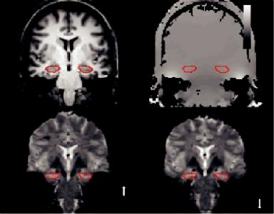
Signal loss can be studied by simulating the effect of field gradients on the EPI signal, and it has been shown (using field maps), that it depends on the image orientation, echo time (TE), and spatial resolution (Ojemann et al., 1997). These acquired field maps can also be used to correct such distortions (Jezzard and Balaban, 1995). Figure 8.1 illustrates an acquired field map along with the reference anatomical image and shows how the choice of phase encoding direction can affect localization accuracy when fieldmap-based distortion compensation techniques are used during data analysis (Olman et al., 2009).
In clinical fMRI, susceptibility artifacts are not limited to anatomical inhomogeneities but can be induced by a number of sources usually related to previous surgery, including clips, stent grafts, etc. Surgery-related materials can induce strong macroscopic field gradients generating appreciable signal losses. Previous surgery can also induce hemorrhages, which can in turn cause susceptibility artifacts, which may degrade pre-surgical fMRI mapping, although in most cases it may still be possible (Peck et al., 2009), keeping in mind that findings should be interpreted with caution in the presence of post-surgical artifacts.
As mentioned earlier, the larger the voxel size, the faster the signal dispersion or signal loss. Hence, fMRI’s spatial resolution is of paramount importance because it is the reduction of voxel size that can reduce the susceptibility effects. Of course, the reduction of voxel size comes at the cost of reduced brain coverage and the question regarding temporal resolution since the dephasing increases with time. In clinical routine, there is a constant tradeoff between spatial and temporal resolution with optimum BOLD phenomenon sensitivity that needs to be accomplished. Echo planar images have an inferior spatial resolution and overall image quality
Artifacts and Pitfalls of fMRI |
|
163 |
(a) |
(b) |
50 |
|
0 Hz
–50
(c) |
(d) |
PE
PE
FIGURE 8.1 (a) Reference ANATOMICAL image for an oblique coronal slice (perpendicular to the hippocampal axis) through the anterior hippocampus (line boundary). (b) Field map (bar indicating frequency offsets in Hz) for the same slice; the ROI boundary is the same as in (a). (c) High resolution, full field of view EPI image with phase-encode (PE) in the foot–head direction. Susceptibility artifacts decrease the static magnetic field in the medial temporal lobe and shift the signal from the PHG toward the feet (notably, the hippocampus is not affected). Increased B0 (static magnetic field strength) in the lateral temporal lobe shifts the signal toward the top of the head. (d) Reversing the phase-encode direction reverses the direction of distortion. The choice of phase-encode direction can affect localization accuracy when field-map-based distortion compensation techniques are used during data analysis. (From Olman, C. A. et al., PLOS One, 4, e8160, 2009.)
than T1 or T2 anatomical scans. The standard maximum resolution of single-shot EPI is about 2 mm2. Nevertheless, one of the most promising developments in fMRI scanner technology has been the use of multiple parallel RF receive coils to help spatially encode the data, thus allowing for much higher resolution with a single excitation pulse, which can allow functional image resolutions of about 1 mm3 (Bandettini, 2009).
Interestingly, it is not the technical limits of the acquisition methods that determine the maximum spatial resolution of the fMRI procedures, but rather the relatively wide spatial spread of the oxygenation and perfusion changes following brain activation, or the so-called “hemodynamic point spread function.” It has been shown that the hemodynamic point spread function of the T2*-weighted gradient echo BOLD response can be of the order of ~3.5 mm at 1.5 T (Engel, 1997), and less than 2 mm at 7 T (Shmuel et al., 2007). Shmuel’s group has also suggested that the point-spread function of T2 and T2* BOLD responses at 7 T relative to metabolic activity have been estimated as ~0.8 mm and ~1.0 mm, respectively (Shmuel and Maier, 2015). Obviously, for a better spatial resolution, the higher the magnetic field the greater the image signal to noise, and the larger the functional contrast, allowing for higher signal per voxel volume.
On the other hand, it has to be mentioned at this point that most fMRI studies involve several techniques and analysis procedures in their data analysis pipeline, that effectively reduce
164 |
Advanced MR Neuroimaging: From Theory to Clinical Practice |
the spatial resolution to about 10 mm3, probably making all the aforementioned efforts for a spatial resolution of less than 2 mm3 potentially redundant. The aforementioned analysis of fMRI data involves multiple stages of data pre-processing before the activation can be statistically detected, such as spatial smoothing, spatial normalization, and multi-subject averaging (Mikl et al., 2008). In other words, high spatial resolution is only absolutely necessary and beneficial when single-subject assessment is involved, where the advantages of collecting high resolution data would yield more subtle and patient specific information.
The hemodynamic response also poses limitations in temporal resolution of the fMRI signals acquired. EPI images have an acquisition window of about 20–30 ms, which relative to the inertia and variability of the hemodynamic response is quite fast and adequate. Nevertheless, the problem arises when the signal is influenced by the underlying vasculature a voxel covers. That is, if a voxel happens to cover large vessel effects, the magnitude of the signal can be up to an order of magnitude larger than the capillary effects and the timing somewhat delayed for up to 4 sec. It follows that signal temporal dynamics varies, and it can generally be described by an increase of the fMRI signal, approximately 2 sec following neuronal activity as well as a plateau in the so-called “on” state for about 7–10 sec (Buxton et al., 2004).
This means that the determination of the precise timing of signal activation between adjacent regions of the brain can be very difficult, and the required temporal resolution to achieve this goal would be of the order of tens of milliseconds.
Several hypotheses have been made regarding the hemodynamic responses of vessels and capillaries, nevertheless the precise mechanisms of these temporal variations are yet to be completely determined. Most hemodynamic response modeling research to date has focused on the magnitude of evoked activation, although timing and shape information should be established first. However, there is a growing interest in measuring onset, peak latency and duration of evoked fMRI responses. A number of fitting procedures exist that potentially allow the characterization of the latency and duration of fMRI responses. Ideally only one model that extracts the shape of the hemodynamic response function (HRF) to different types of cognitive events would be required (Bellgowan et al., 2003; Thompson, Engel, and Olman, 2014). Nevertheless, most groups that analyze functional neuroimaging data assume a fixed shape for the measured response, by regressing data onto a canonical HRF (Smith et al., 2011; Thompson et al., 2014). This approach is widely used, but obviously has limitations because it is unknown whether the timing of fMRI responses changes as neural activity increases (Li et al., 2008; Thompson et al., 2014).
8.2.2 Spatial and Temporal fMRI Resolution—Mitigating Strategies
There are several approaches to increasing fMRI spatial resolution. The most obvious one, as mentioned earlier, is to increase the magnetic field strength, thus increasing the functional signal to noise producing useful data in clinically acceptable times (Murphy et al., 2007). Hence, it is generally recommended and preferable to perform fMRI at 3 T or higher. Especially regarding individual subject assessment, which is by default not spatially smoothed, normalized or averaged, fMRI should only be performed at high magnetic field strengths (≥3 T).
Regarding the mitigation of the hemodynamic point spread function, besides the field strength increase, the primary effort has been to reduce the effects of large vessels, mainly by using spin-echo imaging. Previous evidence showed that, due to refocusing of static dephasing effects around large vessels, spin-echo (SE) BOLD signals offer an increased linearity and promptness with respect to gradient-echo (GE) acquisition, and have been proposed
Artifacts and Pitfalls of fMRI |
165 |
as a potential alternative to obtain increased functional localization to the capillary bed (Chiacchiaretta and Ferretti, 2015; Jochimsen et al., 2004; Norris, 2012; Parkes et al., 2005). In fact, the 180° refocusing pulse that rephases the contribution around larger vessels is also effective at recovering susceptibility effect’s signal loss, making SE sequences superior regarding spatial specificity of the microvasculature but only at high field strengths (≥7 T) (Halai et al., 2014; Schwarzbauer et al., 2010).
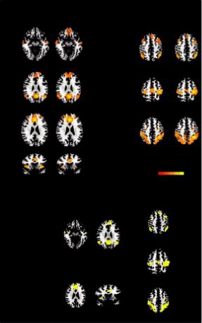
Figure 8.2 shows GE and SE seed-based functional connectivity maps for GE and SE sequences obtained from the random effects group analysis showing resting state networks. It is evident that the spatial patterns were largely overlapping for the two sequences (Figure 8.2b), except for the ventromedial prefrontal cortex of the DMN, which did not show a significant connectivity with the seed in the GE acquisition (Chiacchiaretta and Ferretti, 2015).
DMN
SN
GE and SE functional connectivity maps
GE |
SE |
|
GE |
|
SE |
|
Z = –10 |
|
|
Z = 43 |
|
|
|
ECN |
|
|
|
|
Z = 27 |
|
|
Z = 51 |
|
|
|
SMN |
|
|
|
|
Z = 25 |
|
|
Z = 43 |
|
|
|
DAN |
|
|
|
|
y = 13 |
|
|
|
|
|
|
|
4.1 |
t(15) |
8 |
|
|
|
|
||
|
|
(a) |
|
|
|
|
Overlapping regions of GE and SE |
|
|
||
|
connectivity maps |
z = 43 |
|
||
|
|
|
|
||
|
|
Z = 27 |
|
|
|
|
DMN |
ECN |
z = 51 |
|
|
|
|
|
|
||
|
|
SMN |
|
|
|
|
Z = 25 |
y = 13 |
z = 43 |
|
|
|
SN |
|
|
||
|
DAN |
|
|
|
|
(b)
FIGURE 8.2 Seed-based connectivity maps for gradient-echo (GE) and spin-echo (SE) obtained from the random effects group analysis showing the following resting state networks: default mode network (DMN), executive control network (ECN), salience network (SN), dorsal attention network (DAN), and sensorimotor network (SMN) (a). The group statistical maps were thresholded at p < 0.05, corrected for multiple comparisons using a cluster-size algorithm, and superimposed on the Talairach template; (b) overlapping regions of GE and SE connectivity maps. (From Chiacchiaretta, P. and Ferretti, A., PLOS One, 10, e0120398, 2015.)
166 |
Advanced MR Neuroimaging: From Theory to Clinical Practice |
Another method to increase spatial resolution is an attempt to calibrate the hemodynamic factors that influence the BOLD signal change. For example, differences in the baseline cerebral blood flow and volume, or the rate of breathing and the heart rate might produce variations in the BOLD response (Birn et al., 2006; Thomason and Glover, 2008). Thus, the goal would be to better discriminate fMRI signal components that are related to neural activity from those that result from intrinsic properties of the local vasculature (Thomason and Glover, 2008).
The proposed spatial calibration methods can be described under the general idea of creating a map of potential BOLD signal magnitudes by providing an evenly distributed hemodynamic brain stress such as hypercapnia (Bandettini and Wong, 1997; Thomason et al., 2007) with CO2 inhalation stress (Chiarelli et al., 2007) or Breath Holding (BH) techniques (Handwerker et al., 2007; Thomason et al., 2005).
The map is then used for the correction of vascular reactivity-induced effects in the BOLD signal by dividing activation-induced signal changes, by this map of signal change to the global stress. Measurements taken during stress are used to identify individualand region-specific differences in hemodynamic responsivity, and applying correction for these differences to cognitive paradigms. Very recently CO2 stress and BH calibration techniques have been used to quantify alterations in regional cerebrovascular responsiveness, by applying a global physiological stimulus as a “task” in an effort to assess the cerebrovascular integrity of the entire brain (Gonzales et al., 2014; Mutch et al., 2014).
Regarding temporal resolution the most direct mitigating strategy would be to first positively identify and then remove large vessel effects by using calibration methods, thus reducing physiologic fluctuations and aiming to temporal signal to noise. The major obstacle in comparing the hemodynamic response across systems, and even within systems, is that different brain regions exhibit biologically determined differences (spatial bias) in hemodynamic response properties that are unrelated to the underlying neural function (Bellgowan et al., 2003).
8.2.3 EPI-Related Image Distortions
The main advantage of EPI sequences is that an entire image can be acquired in a fraction of a second practically “freezing” motion during acquisition. Nevertheless, the main drawback of EPI is its high sensitivity to geometric distortions, especially at the boundaries of heterogeneous areas of the brain. This is because there is no such thing as a purely homogeneous magnetic field because even in a perfectly shimmed magnetic field the human head will magnetize unevenly due to air cavities or bone-tissue boundaries, so that the MR frequency may slightly differ from one point to another. These rather small frequency differences (about 1 ppm) unfortunately result in mislocalization of the signal in the phase encoding direction and signal intensity loss in the resulting images.
This signal mislocalization may be a frequent cause of concern in fMRI as the brain activation map is superimposed or fused onto the higher resolution structural images, resulting in improper registration and information errors.
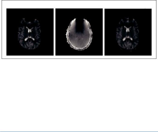
Generally, however, these artifacts may be considerably reduced by distortion correction methods based on the local point spread function (In and Speck, 2012), application of parallel imaging with faster EPI readout using high-performance gradient systems and by image postprocessing. One example of the application of the field map technique, which is one of the most used distortion correction methods, is depicted in Figure 8.3. For an analytical description of
Artifacts and Pitfalls of fMRI |
|
167 |
Distorted EPI Image |
Field Map |
Corrected EPI Image |
FIGURE 8.3 On the left, the distorted (by field inhomogeneity) EPI image is depicted. From the field map image (middle) we get the magnitude of spatial distortions in the phase encoding direction. Then, the field map image is used to calculate distortion and “unwarp” the EPI image, as shown on the right. (Adapted from FSL. Available at https://fsl.fmrib.ox.ac.uk/fsl/fslwiki/ Copyright © 2000-2017, FMRIB Analysis Group and MGH, Boston.)
distortion correction algorithms, (see Hutton et al., 2002) and the more recent review paper by (Jezzard, 2012).
8.3 Physiological Noise and Motion Limitations
Physiological noise and head motion are two patient-related critically important confounds that usually affect the BOLD signal, degrading sensitivity and specificity of the fMRI outcome. When fMRI is performed in the midbrain, motion is a secondary problem compared to the aforementioned susceptibility effects. But this is true only for pulsatile cranio-caudal motion and not for rigid body motion.
Jezzard (1999), defined physiological noise as signal changes that are caused by the subject’s physiology, for example, metabolic and other fluctuations associated with cardiac and respiratory processes, excluding paradigm-related brain activation. The sources of physiological noise in brain fMRI can therefore be identified as both induced by the cardiac and the respiratory cycle. Mechanisms that contribute to noise due to the cardiac cycle are considered to be the changes in cerebral blood flow (CBF) and volume (CBV), arterial pulsatility, and CSF flow (Krüger and Glover, 2001), while mechanisms that contribute to noise due to the respiratory cycle include induced changes in arterial CO2 partial pressure (Wise et al., 2004), and possible changes in the main magnetic field (B0) (Raj et al., 2001).
These mechanisms affect the fMRI signal in different ways, but generally, bulk motion will lead to similar artifacts as rigid body head motion. For instance, the magnetic field can be altered either by the movement of the subject’s chest (Brosch et al., 2002) or by susceptibility induced changes in the lungs (Raj et al., 2001), leading to apparent movement due to the geometric distortion associated with the varying magnetic field. These magnetic field changes usually result in a shift of the MR image in the phase-encoding direction and the displacements of voxels in the image cause artifacts that are particularly harmful near
168 |
Advanced MR Neuroimaging: From Theory to Clinical Practice |
areas with high susceptibility differences, such as at the edge of the brainstem (Brooks et al., 2013). Other mechanisms such as oxygenation or blood volume changes create alterations in local blood susceptibility, and these changes will induce BOLD-related signal variations in the same pattern as the expected brain activations induced by paradigms. Breathing can also affect the head motion, which may spatially alter spin history (Friston et al., 1996) and, along with cardiac pulsation, can cause the brain stem to push up into the surrounding brain tissue. In either case, the main magnetic field is altered by the deformation and cerebrospinal fluid movement (Dagli et al., 1999). There are also ways that the signal can be affected via changes in tissue composition or via inflow effects (Brooks et al., 2013). That is, vessel’s pulsations that are generated by cardiac-induced pressure changes may produce small movements in and around large blood vessels (Dagli et al., 1999). In any case, Soellinger et al. (2007) reported a heartbeat-correlated pulsatile cranio-caudal motion of no more than 0.2-mm displacements with peak velocities ≤2 mm/s.
It is very interesting to mention here that all the aforementioned mechanisms of physiological noise are field strength dependent. Moreover, while the signal-to-noise ratio (SNR) increases linearly with field strength, the relative contribution of physiological noise increases with the square of the field (Triantafyllou et al., 2005). Consequently, strategies for reducing the effects of physiological fluctuations are particularly important in fMRI studies at higher field strengths such as 7 T because physiological noise can become the dominant source of noise, giving rise to false positive activations. Especially for subtle BOLD responses, it is of paramount importance to increase the temporal SNR (tSNR) by the use of optimal physiological noise correction methods (Hutton et al., 2011).
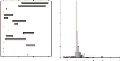
Indicatively, an overview of the SNR values that were reported for real fMRI data from a recent study are presented in Figure 8.4. Many authors explicitly reported tSNR values ranging from 4.42 to 280, while in a few other cases, the CNR values that were reported varied from 0.5 to 1.8. Both in the experimental and simulation studies in this literature search, the reported values demonstrated a range that was much wider than can be explained by natural variation only (Welvaert and Rosseel, 2013).
Reported SNR values based on real data
Koush et al. Van Dijk et al.
Conijn et al. Scholvinck et al.
Newton et al. Hahn and Rowe Bungert et al. Shen et al. Sarkka et al. Lopes et al. Posse et al. Hughes and Beer Janssens et al. Yang et al. Zotev et al. Beckett et al.
Ing and Schwarzbauer Driver et al.
0 50 100 150 200 250 300 SNR/CNR
Histogram of SNR values reported in simulation studies
0 20 40 60 80 100
–10 |
0 |
10 |
20 |
30 |
40 |
50 |
FIGURE 8.4 Overview of reported SNR values in real data (left panel) and simulated data (right panel). (From Welvaert, M. and Rosseel, Y., PLOS One, 8, e77089, 2013.)
Artifacts and Pitfalls of fMRI |
169 |
8.3.1 Physiological Noise—Mitigating Strategies
Several different mitigating strategies have been proposed to minimize the influence of physiological noise in fMRI experiments, broadly falling into the following categories:
1.Gating (cardiac or respiratory), referring to techniques that attempt to effectively “freeze” physiological motion (prospective techniques)
2.Acquisition-based image corrections, referring to techniques aiming to correct for signal intensity variations
3.Calibration, referring to techniques that include additional scans to identify noise sources and retrospectively eliminate them (retrospective techniques)
8.3.1.1 Cardiac Gating
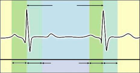
Cardiac pulsations can induce temporal signal fluctuations, and it has been shown that within a cardiac cycle, brain tissue (particularly at the base of the brain) can move up to a range of several millimeters. Cardiac gating ensures that an image is collected at the same phase of each cardiac cycle, typically by phase locking the sampling to a fixed time point during each cardiac cycle ensuring that the images are repeatedly registered, as this is illustrated in Figure 8.5.
The only drawback is that the heart rate can be variable, hence the TR will no longer be “fixed” but it will vary accordingly. A cardiac cycle dependent TR will lead to large signal variations due to varying longitudinal (T1) saturation, meaning that that there will be different amounts of T1 relaxation between samples. This problem has to be accounted for and corrected.
There are two approaches regarding this correction. The first approach is to use an effective TR so that the extra amount of partial saturation of the MR signal is corrected (increased or decreased appropriately) by an adjustment of the intermediate time between samples (Malinen et al., 2006). Nevertheless, additional processing is required to minimize induced effects of a variable TR, such as a lack of information on the relative magnitude of cardiac noise, or a difficulty to accurately correct for the signal variations due to the alteration of repetition time.
Target R-R Interval
Trigger |
Trigger |
Acquisition window |
Trigger |
Trigger |
|
||||
window |
delay |
|
window |
delay |
FIGURE 8.5 Cardiac gating ensures that an image is collected at the same phase of the cardiac cycle, typically by phase locking the sampling to a particular time point during each cardiac cycle.
170 |
Advanced MR Neuroimaging: From Theory to Clinical Practice |
The second approach is to acquire gated imaging data with a minimum of two echoes per repetition time (TR) in order to derive an image basically reflecting T2* effects, thus reducing signal variations due to T1 saturation effects (Beissner et al., 2010; Beissner et al., 2011; Zhang et al., 2006). The technique is based on the calculation of the apparent T2* using a mathematical approach, or by computing the quotient of every two images per repetition time. In any case, according to Breissner et al. (2011), pre-processing for the smoothing of data and optimal normalization is necessary.
8.3.1.2 Acquisition-Based Image Corrections
Physiologically-induced image artifacts can be mitigated using modifications of the pulse sequence parameters of BOLD imaging, although the major difficulty that arises, is to maintain an adequately high SNR. As mentioned earlier, the EPI acquisitions that are typically used for fMRI are vulnerable to phase errors from field variations due to motion and hence multiple variations of the T2*-weighted sequences have been proposed to resolve these issues, such as multi-echo EPI and parallel imaging acquisitions using slice-dependent TE sequences. Especially at higher magnetic fields (>3 T) these can be easily implemented as modified versions of Gradient Echo sequences, using multi-channel coils (Domsch et al., 2013; Zaca et al., 2014).
The multi-channel array coils with parallel imaging may increase the contrast to noise ratio of the EPI data using reduced echo train lengths to acquire additional echoes for the same TR. It has been shown that multi-echo imaging techniques can minimize physiological signal fluctuation in and around the brainstem (Kundu et al., 2012).
Another approach to minimizing the influences of geometric distortions is the use of the Point Spread Function (PSF) (Zaitsev et al., 2004). Additional phase encoding gradient acquisitions in the x, y, and z directions are used to map all three-dimensional PSFs of each voxel. Then PSFs are used to describe each voxel’s distribution of intensities and hence spatial information, which allows the geometrical distortion to be corrected for. The downside is that this technique obviously requires additional scan and processing times, limiting its use in clinical routine.
The last popular imaging technique to mitigate these influences is the use of the so-called “navigator echoes” (Pfeuffer et al., 2002). The general idea is to acquire an additional non-phase-encoded navigator echo before the image read-out in order to adjust the phase shift of the data produced by the motion-induced time-varying magnetic field. The comparison of the navigator echo to the central line of the main k-space data then be used to correct the phase of all other echoes recorded and yield enough information to remove the geometric distortion in the phase-encoding direction. Nevertheless, caution is needed since navigator echoes are not so easy to manipulate.
8.3.1.3 Calibration
8.3.1.3.1 Calibration Scans
The idea behind calibration scans is to record and identify physiological signals in the absence of any external brain stimulation and then remove them from the task fMRI results during the data post-processing. The procedure is sometimes called a “clean-up” since it utilizes the physiological recordings to remove the estimates from each voxel’s time series using linear regression, thus “cleaning up” the fMRI data (Murphy et al., 2013). This is done using a linear regression procedure to model the BOLD signal as a time series, and to fit it to the “influenced” data. This fit is then subtracted from the original data to remove the associated physiological variance.
While this approach increases the effectiveness of fMRI experiments, there are some associated disadvantages, such as (1) the extra time needed to acquire the additional scan for the

Artifacts and Pitfalls of fMRI |
171 |
calibration, and more importantly (2) the possibility of removing signals that are recognized as physiological noise but may be indeed signals correlated to the induced brain function.
The same goal of physiological noise sources removal can be mitigated by several approaches and in different data levels. Hu et al. (1995) proposed a method to retrospectively estimate and correct the primary fluctuation effects of cardiac and respiratory cycles using pulse oximeters and respiratory bellows in the k-space (called RETROKCOR), while Glover et al. (2000) proposed the same approach but in the image space data and argued that for standard acquisitions it worked better than the k-space approach (called RETROCOIR). This is most probably due to the fact that corrections of single k-space points affect all voxels, potentially introducing spatially correlated noise in all data (Murphy et al., 2013).
Both the RETROKCOR from Hu et al., and the RETROCOIR from Glover et al., obviously depend on the model used to approximate the physiological fluctuations effects. These signal fluctuations can alternatively be reduced by the use of a model-free adaptive filtering, provided they are repetitive and their timing is known (Deckers et al., 2006). The performance of this approach has been proposed to be at least equivalent to the RETROCOIR method, under the assumption that “each occurrence of the quasi-periodic disturbance (‘event’) leads to an artifact with spatial and temporal signal perturbation characteristics that only depend on the timing of the event relative to MRI data acquisition” (Deckers et al., 2006).
There are also a number of pre-processing strategies used for reducing physiological noise implemented after the acquisition, including (1) temporal filtering (theoretically, it is possible to filter and remove signals with certain frequencies, such as the cardiac and respiratory cycle) and (2) denoising with independent component analysis (ICA) (theoretically, using machine learning algorithms and automated classification methods, any dataset can be “cleaned up” or decomposed into its constituent sources). Nevertheless, a potential limitation regarding temporal filtering is that the acquisition rate of fMRI data does not adequately sample the cardiac and respiratory variations that might be aliased into the BOLD signal frequency (Zaca et al., 2014). Hence, removing physiological noise will also remove portions of the BOLD processes, decreasing the overall signal. To this effect, special attention must be given in the subsequent statistics when denoising with ICA in order to avoid falsely inflated statistics (Brooks et al., 2013).
Eventually the question that arises is: which one should be used?
Unfortunately, there is not an easy answer. It depends on various factors, such as the subject group, the available software and scanner, as well as the specific fMRI experiment.
Overall there are several different “ready-to-use” software packages for physiological noise mitigation of fMRI data, either as specific tools embedded in other software, or as stand-alone packages. As an indication these are illustrated (but not limited to) in the following updated table (Table 8.1) including data from Brooks et al. (2013). For the interested reader, the review paper by Brooks et al. (2013) provides extended information and details for physiological noise in brainstem fMRI.
8.4 Interpretation Limitations
Probably the major concern raised with respect to the interpretation of BOLD fMRI is the uncertainty of neural activity localization. The fundamental goal in fMRI is to be able to precisely detect transient hemodynamic changes involving a number of mechanisms following neuronal activation, such as changes in blood flow, volume, and oxygenation. The uncertainty

172 Advanced MR Neuroimaging: From Theory to Clinical Practice
TABLE 8.1 A Selection of Software Packages for Physiological Noise Mitigation and Processing of fMRI Data
TOOLS |
URL |
|
|
Stand-Alone Packages |
|
RETROICOR tool |
http://www.mccauslandcenter.sc.edu/crnl/tools/part |
PART (Physiological Artifact Removal Tool) |
http://journals.plos.org/plosone/article?id=10.1371 |
|
/journal.pone.0001751#pone.0001751.s001 |
PhysioNoise |
https://github.com/timothyv |
|
/Physiological-Log-Extraction-for-Modeling |
|
--PhLEM--Toolbox |
PhLEM (Physiological Log Extraction for Modeling) |
https://www.tnu.ethz.ch/de/software/tapas.html |
TAPAS PhyslO Toolbox |
http://www.cs.tut.fi/~jupeto/software.html |
ICA Artifact Remover NIAK (NeuroImaging |
http://www.mrijournal.com/article/S0730 |
Analysis Kit) |
-725X(06)00342-0/abstract |
CORSICA (CORrection of Structured noise using |
http://www.nitrc.org/projects/pestica |
spatial Independent Component Analysis) |
|
PESTICA (Physiologic EStimation by Temporal ICA) |
http://cbi.nyu.edu/software/ |
Specific Tools |
|
RETROICOR (RETROspective Image CORrection) |
http://afni.nimh.nih.gov/pub/dist/doc/program |
(AFNI) |
_help/3dretroicor.html |
RETROICOR (FreeSurfer) |
https://github.com/neurodebian/freesurfer/blob |
|
/master/fsfast/toolbox/fast_retroicor.m |
DRIFTER (Dynamic RetrospectIve FilTERing) (SPM |
http://becs.aalto.fi/en/research/bayes/drifter/ |
ToolBox) |
|
PNM (physiological noise model) (Part of FSL) |
http://fsl.fmrib.ox.ac.uk/fsl/fslwiki/PNM |
FIX (FMRIB’s ICA-based X-noisifier) (Part of FSL) |
http://fsl.fmrib.ox.ac.uk/fsl/fslwiki/FIX |
Processing Software |
|
AFNI (Analysis of Functional NeuroImages) |
https://afni.nimh.nih.gov/ |
BrainVoyager (analysis and visualization of structural |
http://www.brainvoyager.com/ |
and functional magnetic resonance imaging data) |
|
FMRISTAT (A general statistical analysis for fMRI |
http://www.math.mcgill.ca/keith/fmristat/ |
data) (From McGill University) |
|
BIC (Brain Imaging Centre) Software |
https://www.mcgill.ca/bic/software |
Brain Connectivity Toolbox (Most widely used to |
https://sites.google.com/site/bctnet/ |
analyze resting-state fMRI studies) |
|
BrainSuite (A collection of open source software |
http://brainsuite.org/ |
tools) |
|
BrainVISA (A free neuroimaging software platform |
http://www.brainvoyager.com/ |
for mass data analysis) (IFR-France) |
|
FreeSurfer is an open source software suite for |
http://www.brainvoyager.com/ |
processing and analyzing brain MR images |
|
FSL (FMRIB Software Library) |
https://fsl.fmrib.ox.ac.uk/fsl/fslwiki/ |
SPM (Statistical Parametric Mapping) |
http://www.fil.ion.ucl.ac.uk/spm/ |
REST (RESting-state fMRI data analysis Toolkit) is a |
http://restfmri.net/forum/index.php?q=rest |
group of applications based on MATLAB and SPM8 |
|
for evaluation of resting-state fMRI data |
|
MIALAB (Medical Image Analysis Lab) |
http://mialab.mrn.org/ |
|
|

Artifacts and Pitfalls of fMRI |
173 |
arises from the fact that the extent of the fMRI hemodynamic response around the active sites, at submillimeter resolution, remains controversial (Duong et al., 2000; Zaca et al., 2014).
Why?
The explanation is that these hemodynamic changes can propagate from the capillary beds adjacent to the site of neuronal activation beyond the actual activated sites, hence the BOLD response may appear diffused far from the active sites (Duong et al., 2000; Duong et al., 2001).
In fact, we need to realize that the BOLD contrast arises from a complex interplay between cerebral blood flow, cerebral blood volume, and cerebral metabolic rate of oxygen consumption on a spatial scale that lumps together hundreds of thousands of neurons in each MR imaging voxel (Zaca et al., 2014). In that sense, it is very much dependent on the local vasculature and its spatial characteristics (Kim and Ogawa, 2012; Moon et al., 2013), and obviously depends on the area of activation. More specifically, the spatial specificity can be decreased because of the so-called venous effects. Especially in areas of high vascular density, these effects increase the probability of false-positive activation since the strongest BOLD signal change is generated near draining veins (Bianciardi et al., 2011). Nevertheless, at the increasingly high magnetic fields used clinically, spatial resolution can be improved using spin-echo sequences (Kim and Ogawa, 2012). Especially with the introduction of ultrahigh field magnets (>7 T), susceptibility weighted imaging has been used to remove the venous signal, in terms of vascular activation masking. Then, the venous contribution is expected to decrease since, with higher magnetic fields and longer TEs, the extravascular contribution increases and the intravascular contribution decreases; therefore, the spatial specificity to parenchyma improves (Kim and Ogawa, 2012). Another approach to increasing the spatial specificity is to enhance the statistical significance threshold. However, this might cause the opposite error of false-negative activation since the background signal might wash out and should be avoided.
The extent of activation foci is limited by another difficulty, which relates to the high interand intra-subject variability observed with fMRI, even with constant scanning parameters and consistent task performance (Goodyear et al., 2014). Especially regarding fMRI pre-surgical mapping, perhaps the most serious concern is the lack of systematic establishment and verification of the technique in different patient types and using specific activation paradigms.
Again, the extent of activation depends on a statistical threshold, which in turn is determined by the quality of the BOLD signal and the accomplished SNR. This is called activation map thresholding, and it has been shown that although the spatial distribution of BOLD t-value statistical activation maps can be highly variable across subjects and scan duration, the use of relative activation maps, (e.g., the use of 40% of the most active voxels) resulted in highly reproducible results both within individual subjects and across different subjects (Voyvodic et al., 2009).
8.5 Quality Assurance in fMRI
All MRI studies should be performed in a well-maintained scanner and a quality assurance (QA) program should be mandatory to obtain optimal images in any clinical environment. fMRI studies are particularly demanding and should be given extra attention since they utilize fast imaging methods such as echo-planar imaging (EPI) or spiral acquisitions that usually push the scanner hardware to its limits. Hence, besides good experimental design, correct
174 |
Advanced MR Neuroimaging: From Theory to Clinical Practice |
technical execution of the scan and minimal subject and physiological motion, the fMRI experiment should include a well-designed QA program to ensure optimal data extraction.
There are several specifically designed QA programs for fMRI studies and the interested reader should refer to them for an analytical description and guidance. (Friedman and Glover, 2006; Greve et al., 2011; Olsrud et al., 2008; Stöcker et al., 2005; Sutton et al., 2008). Nevertheless, it is important that each research site establish its own QA performance criteria and the aforementioned QA studies may be useful in guiding the establishment of such criteria. Ideally, fMRI QA scans should be run daily and a good recommended practice is to have the QA scans acquired at the beginning of each day prior to any scheduled scans.
8.6 Conclusion
Functional MRI has made a huge clinical impact during the last decade for the noninvasive evaluation of brain functionality and connectivity, and it is safe to argue that in the following years it may further improve the effectiveness of human brain studies in an accelerated fashion.
Nevertheless, there should be an even greater degree of attention to the data analysis methods and the new acquisition protocols used since, undoubtedly, there are many issues that need to be resolved before clinical fMRI can be fully implemented in the clinical routine. Although the vast majority of fMRI studies are carefully conducted, the correct and consistent application of the analysis pipeline can often be very challenging. All fMRI studies will continuously strike a delicate balance between over-analyzing or underestimating the results, as well as put forth a continuous effort to recognize and cope with technical and physiological artifacts and sources of error.
References
Bandettini, P. A. (2009). Functional MRI limitations and aspirations. In E. Poppel, B. Gulyas, E. Kraft, A. Muller, and E. Poppel (Eds.), Neural Correlates of Thinking. Berlin, Heidelberg: Springer.
Bandettini,P.A.andWong,E.C.(1997).Ahypercapnia-basednormalizationmethodforimproved spatial localization of human brain activation with fMRI. NMR in Biomedicine, 10(4–5), 197–203. doi:10.1002/(sici)1099-1492(199706/08)10:4/5<197::aid-nbm466>3.0.co;2-s
Beissner, F., Baudrexel, S., Volz, S., and Deichmann, R. (2010). Dual-echo EPI for non-equi- librium fMRI—Implications of different echo combinations and masking procedures. NeuroImage, 52(2), 524–531. doi:10.1016/j.neuroimage.2010.04.243
Beissner, F., Deichmann, R., and Baudrexel, S. (2011). FMRI of the brainstem using dual-echo EPI. NeuroImage, 55(4), 1593–1599. doi:10.1016/j.neuroimage.2011.01.042
Bellgowan, P. S., Saad, Z. S., and Bandettini, P. A. (2003). Understanding neural system dynamics through task modulation and measurement of functional MRI amplitude, latency, and width. Proceedings of the National Academy of Sciences, 100(3), 1415–1419. doi:10.1073/ pnas.0337747100
Bianciardi, M., Fukunaga, M., Gelderen, P. V., Zwart, J. A., and Duyn, J. H. (2011). Negative BOLD-fMRI signals in large cerebral veins. Journal of Cerebral Blood Flow & Metabolism, 31(2), 401–412. doi:10.1038/jcbfm.2010.164
Birn, R. M., Diamond, J. B., Smith, M. A., and Bandettini, P. A. (2006). Separating respira- tory-variation-related fluctuations from neuronal-activity-related fluctuations in fMRI. NeuroImage, 31(4), 1536–1548. doi:10.1016/j.neuroimage.2006.02.048
Brooks, J. C., Faull, O. K., Pattinson, K. T., and Jenkinson, M. (2013). Physiological noise in brainstem fMRI. Frontiers in Human Neuroscience, 7, 623. doi:10.3389/fnhum.2013.00623
Artifacts and Pitfalls of fMRI |
175 |
Brosch, J., Talavage, T., Ulmer, J., and Nyenhuis, J. (2002). Simulation of human respiration in fMRI with a mechanical model. IEEE Transactions on Biomedical Engineering, 49(7), 700–707. doi:10.1109/tbme.2002.1010854
Buxton, R. B., Uludağ, K., Dubowitz, D. J., and Liu, T. T. (2004). Modeling the hemodynamic response to brain activation. NeuroImage, 23, Suppl 1, S220–233. doi:10.1016/j. neuroimage.2004.07.013
Chiacchiaretta, P. and Ferretti, A. (2015). Resting state BOLD functional connectivity at 3T: Spin echo versus gradient echo EPI. PLOS One, 10(3), e0120398. doi:10.1371/journal.pone.0120398 Chiarelli, P. A., Bulte, D. P., Wise, R., Gallichan, D., and Jezzard, P. (2007). A calibration method for quantitative BOLD fMRI based on hyperoxia. NeuroImage, 37(3), 808–820. doi:10.1016/j.
neuroimage.2007.05.033
Dagli, M. S., Ingeholm, J. E., and Haxby, J. V. (1999). Localization of cardiac-induced signal change in fMRI. NeuroImage, 9(4), 407–415. doi:10.1006/nimg.1998.0424
Deckers, R. H., Gelderen, P. V., Ries, M., Barret, O., Duyn, J. H., Ikonomidou, V. N., and Zwart, J. A. (2006). An adaptive filter for suppression of cardiac and respiratory noise in MRI time series data. NeuroImage, 33(4), 1072–1081. doi:10.1016/j.neuroimage.2006.08.006
Domsch, S., Linke, J., Heiler, P. M., Kroll, A., Flor, H., Wessa, M., and Schad, L. R. (2013).
Increased BOLD sensitivity in the orbitofrontal cortex using slice-dependent echo times at 3T. Magnetic Resonance Imaging, 31(2), 201–211. doi:10.1016/j.mri.2012.06.020
Duong, T. Q., Kim, D., Uğurbil, K., and Kim, S. (2000). Spatiotemporal dynamics of the BOLD fMRI signals: Toward mapping submillimeter cortical columns using the early negative response. Magnetic Resonance in Medicine, 44(2), 231–242. doi:10.1002/1522-2594(200008)44:2<231::aid-mrm10>3.3.co;2-k
Duong, T. Q., Kim, D., Uğurbil, K., and Kim, S. (2001). Localized cerebral blood flow response at submillimeter columnar resolution. Proceedings of the National Academy of Sciences,
98(19), 10904–10909. doi:10.1073/pnas.191101098
Engel, S. (1997). Retinotopic organization in human visual cortex and the spatial precision of functional MRI. Cerebral Cortex, 7(2), 181–192. doi:10.1093/cercor/7.2.181
Friedman, L. and Glover, G. H. (2006). Report on a multicenter fMRI quality assurance protocol. Journal of Magnetic Resonance Imaging, 23(6), 827–839. doi:10.1002/jmri.20583
Friston, K. J., Williams, S., Howard, R., Frackowiak, R. S., and Turner, R. (1996). Movementrelated effects in fMRI time-series. Magnetic Resonance in Medicine, 35(3), 346–355. doi:10.1002/mrm.1910350312
Glover, G. H., Li, T., and Ress, D. (2000). Image based method for retrospective correction of physiological motion effects in fMRI: RETROICOR. Magnetic Resonance in Medicine, 44(1), 162–167. doi:10.1002/1522-2594(200007)44:1<162::aid-mrm23>3.3.co;2-5
Gonzales, M. M., Tarumi, T., Mumford, J. A., Ellis, R. C., Hungate, J. R., Pyron, M., and Haley, A. P. (2014). Greater BOLD response to working memory in endurance-trained adults revealed by breath-hold calibration. Human Brain Mapping, 35(7), 2898–2910. doi:10.1002/hbm.22372
Goodyear, B., Liebenthal, E., and Mosher, V. (2014). Active and passive fMRI for presurgical mapping of motor and language cortex. In T. D. Papageorgiou, G. I. Christopoulos, and S. M. Smirnakis (Eds.), Advanced Brain Neuroimaging Topics in Health and Disease—Methods and Applications. doi:10.5772/58269
Greve, D. N., Mueller, B. A., Liu, T., Turner, J. A., Voyvodic, J., Yetter, E. et al. (2011). A novel method for quantifying scanner instability in fMRI. Magnetic Resonance in Medicine, 65(4), 1053–1061. doi:10.1002/mrm.22691
Halai, A. D., Welbourne, S. R., Embleton, K., and Parkes, L. M. (2014). A comparison of dual gradient-echo and spin-echo fMRI of the inferior temporal lobe. Human Brain Mapping, 35(8), 4118–4128. doi:10.1002/hbm.22463
176 |
Advanced MR Neuroimaging: From Theory to Clinical Practice |
Handwerker, D. A., Gazzaley, A., Inglis, B. A., and Desposito, M. (2007). Reducing vascular variability of fMRI data across aging populations using a breathholding task. Human Brain Mapping, 28(9), 846–859. doi:10.1002/hbm.20307
Hu, X., Le, T. H., Parrish, T., and Erhard, P. (1995). Retrospective estimation and correction of physiological fluctuation in functional MRI. Magnetic Resonance in Medicine, 34(2), 201–212. doi:10.1002/mrm.1910340211
Hutton, C., Bork, A., Josephs, O., Deichmann, R., Ashburner, J., and Turner, R. (2002). Image distortion correction in fMRI: A quantitative evaluation. NeuroImage, 16(1), 217–240. doi:10.1006/nimg.2001.1054
Hutton, C., Josephs, O., Stadler, J., Featherstone, E., Reid, A., Speck, O., and Weiskopf, N. (2011). The impact of physiological noise correction on fMRI at 7T. NeuroImage, 57(1), 101–112. doi:10.1016/j.neuroimage.2011.04.018
In, M. and Speck, O. (2012). Highly accelerated PSF-mapping for EPI distortion correction with improved fidelity. MAGMA, 25(3), 183–192.
Jezzard, P. (1999). Physiological noise: Strategies for correction. In C. Moonen, P. A. Bandettini (Eds.), Functional MRI (pp. 171–179). Heidelberg, Germany: Springer-Verlag.
Jezzard, P. (2012). Correction of geometric distortion in fMRI data. NeuroImage, 62(2), 648–651. doi:10.1016/j.neuroimage.2011.09.010
Jezzard, P. and Balaban, R. S. (1995). Correction for geometric distortion in echo planar images from B0 field variations. Magnetic Resonance in Medicine, 34(1), 65–73. doi:10.1002/ mrm.1910340111
Jochimsen, T. H., Norris, D. G., Mildner, T., and Möller, H. E. (2004). Quantifying the intraand extravascular contributions to spin-echo fMRI at 3 T. Magnetic Resonance in Medicine,
52(4), 724–732. doi:10.1002/mrm.20221
Kim, S. and Ogawa, S. (2012). Biophysical and physiological origins of blood oxygenation leveldependent fMRI signals. Journal of Cerebral Blood Flow and Metabolism, 32(7), 1188–1206. doi:10.1038/jcbfm.2012.23
Krüger, G. and Glover, G. H. (2001). Physiological noise in oxygenation sensitive magnetic resonance imaging. Magnetic Resonance in Medicine, 46(4), 631–637. doi:10.1002/mrm.1240.abs Kundu, P., Inati, S. J., Evans, J. W., Luh, W., and Bandettini, P. A. (2012). Differentiating BOLD and non-BOLD signals in fMRI time series using multi-echo EPI. NeuroImage, 60(3),
1759–1770. doi:10.1016/j.neuroimage.2011.12.028
Li, X., Lu, Z., Tjan, B. S., Dosher, B. A., and Chu, W. (2008). Blood oxygenation level-depen- dent contrast response functions identify mechanisms of covert attention in early visual areas. Proceedings of the National Academy of Sciences, 105(16), 6202–6207. doi:10.1073/ pnas.0801390105
Malinen, S., Schürmann, M., Hlushchuk, Y., Forss, N., and Hari, R. (2006). Improved differentiation of tactile activations in human secondary somatosensory cortex and thalamus using cardiac-triggered fMRI. Experimental Brain Research, 174(2), 297–303. doi:10.1007/ s00221-006-0465-z
Mikl, M., Mareček, R., Hluštík, P., Pavlicová, M., Drastich, A., Chlebus, P. et al. (2008). Effects of spatial smoothing on fMRI group inferences. Magnetic Resonance Imaging, 26(4), 490– 503. doi:10.1016/j.mri.2007.08.006
Moon, C. H., Fukuda, M., and Kim, S. (2013). Spatiotemporal characteristics and vascular sources of neural-specific and -nonspecific fMRI signals at submillimeter columnar resolution. NeuroImage, 64, 91–103. doi:10.1016/j.neuroimage.2012.08.064
Artifacts and Pitfalls of fMRI |
177 |
Murphy, K., Birn, R. M., and Bandettini, P. A. (2013). Resting-state fMRI confounds and cleanup. NeuroImage, 80, 349–359. doi:10.1016/j.neuroimage.2013.04.001
Murphy, K., Bodurka, J., and Bandettini, P. A. (2007). How long to scan? The relationship between fMRI temporal signal to noise ratio and necessary scan duration. NeuroImage, 34(2), 565–574. doi:10.1016/j.neuroimage.2006.09.032
Mutch, W. A., Ellis, M. J., Graham, M. R., Wourms, V., Raban, R., Fisher, J. A., and Ryner, L. (2014). Brain MRI CO2 stress testing: A pilot study in patients with concussion. PLOS One, 9(7), e102181. doi:10.1371/journal.pone.0102181
Norris, D. G. (2006). Principles of magnetic resonance assessment of brain function. Journal of Magnetic Resonance Imaging, 23(6), 794–807. doi:10.1002/jmri.20587
Norris, D. G. (2012). Spin-echo fMRI: The poor relation? NeuroImage, 62(2), 1109–1115. doi:10.1016/j.neuroimage.2012.01.003
Ojemann, J. G., Akbudak, E., Snyder, A. Z., Mckinstry, R. C., Raichle, M. E., and Conturo, T. E. (1997). Anatomic localization and quantitative analysis of gradient refocused echo-planar fMRI susceptibility artifacts. NeuroImage, 6(3), 156–167. doi:10.1006/nimg.1997.0289
Olman, C. A., Davachi, L., and Inati, S. (2009). Distortion and signal loss in medial temporal lobe. PLOS One, 4(12), e8160. doi:10.1371/journal.pone.0008160
Olsrud, J., Nilsson, A., Mannfolk, P., Waites, A., and Ståhlberg, F. (2008). A two-compartment gel phantom for optimization and quality assurance in clinical BOLD fMRI. Magnetic Resonance Imaging, 26(2), 279–286. doi:10.1016/j.mri.2007.06.010
Parkes, L. M., Schwarzbach, J. V., Bouts, A. A., Deckers, R. H., Pullens, P., Kerskens, C. M., and Norris, D. G. (2005). Quantifying the spatial resolution of the gradient echo and spin echo BOLD response at 3 Tesla. Magnetic Resonance in Medicine, 54(6), 1465–1472. doi:10.1002/ mrm.20712
Peck, K. K., Bradbury, M., Petrovich, N., Hou, B. L., Ishill, N., Brennan, C., and Holodny, A. I. (2009). Presurgical evaluation of language using functional magnetic resonance imaging in brain tumor patients with previous surgery. Neurosurgery, 64(4), 644–653. doi:10.1227/01. neu.0000339122.01957.0a
Pfeuffer, J., Moortele, P. V., Ugurbil, K., Hu, X., and Glover, G. H. (2002). Correction of physiologically induced global off-resonance effects in dynamic echo-planar and spiral functional imaging. Magnetic Resonance in Medicine, 47(2), 344–353. doi:10.1002/ mrm.10065
Raj, D., Anderson, A. W., and Gore, J. C. (2001). Respiratory effects in human functional magnetic resonance imaging due to bulk susceptibility changes. Physics in Medicine and Biology, 46(12), 3331–3340. doi:10.1088/0031-9155/46/12/318
Schwarzbauer, C., Mildner, T., Heinke, W., Brett, M., and Deichmann, R. (2010). Dual echo EPI—The method of choice for fMRI in the presence of magnetic field inhomogeneities? NeuroImage, 49(1), 316–326. doi:10.1016/j.neuroimage.2009.08.032
Shmuel, A. and Maier, A. (2015). Locally measured neuronal correlates of functional MRI signals. In K. Ugurbil, L. Berliner, and K. Uludag (Eds.), FMRI: From Nuclear Spins to Brain Functions. New York, NY: Springer.
Shmuel, A., Yacoub, E., Chaimow, D., Logothetis, N. K., and Ugurbil, K. (2007). Spatio-temporal point-spread function of fMRI signal in human gray matter at 7 Tesla. NeuroImage, 35(2), 539–552. doi:10.1016/j.neuroimage.2006.12.030
Smith, S. M., Beckmann, C. F., Khorshidi, G. S., Miller, K. L., Nichols, T. E., Ramsey, J. et al. (2011). Network modelling methods for FMRI. NeuroImage, 54(2), 875–891.
178 |
Advanced MR Neuroimaging: From Theory to Clinical Practice |
Soellinger, M., Ryf, S., Boesiger, P., and Kozerke, S. (2007). Assessment of human brain motion using CSPAMM. Journal of Magnetic Resonance Imaging, 25(4), 709–714. doi:10.1002/ jmri.20882
Stöcker, T., Schneider, F., Klein, M., Habel, U., Kellermann, T., Zilles, K., and Shah, N. J. (2005). Automated quality assurance routines for fMRI data applied to a multicenter study. Human Brain Mapping, 25(2), 237–246. doi:10.1002/hbm.20096
Sutton, B. P., Goh, J., Hebrank, A., Welsh, R. C., Chee, M. W., and Park, D. C. (2008). Investigation and validation of intersite fMRI studies using the same imaging hardware. Journal of Magnetic Resonance Imaging, 28(1), 21–28. doi:10.1002/jmri.21419
Thomason, M. E., Burrows, B. E., Gabrieli, J. D., and Glover, G. H. (2005). Breath holding reveals differences in fMRI BOLD signal in children and adults. NeuroImage, 25(3), 824–837. doi:10.1016/j.neuroimage.2004.12.026
Thomason, M. E., Foland, L. C., and Glover, G. H. (2007). Calibration of BOLD fMRI using breath holding reduces group variance during a cognitive task. Human Brain Mapping, 28(1), 59–68.
Thomason, M. E. and Glover, G. H. (2008). Controlled inspiration depth reduces variance in breath-holding-induced BOLD signal. NeuroImage, 39(1), 206–214.
Thompson, S. K., Engel, S. A., and Olman, C. A. (2014). Larger neural responses produce BOLD signals that begin earlier in time. Frontiers in Neuroscience, 8, 159. doi:10.3389/ fnins.2014.00159
Triantafyllou, C., Hoge, R., Krueger, G., Wiggins, C., Potthast, A., Wiggins, G., and Wald, L. (2005). Comparison of physiological noise at 1.5 T, 3 T and 7 T and optimization of fMRI acquisition parameters. NeuroImage, 26(1), 243–250. doi:10.1016/j.neuroimage.2005.01.007 Voyvodic, J. T., Petrella, J. R., and Friedman, A. H. (2009). FMRI activation mapping as a percentage of local excitation: Consistent presurgical motor maps without threshold adjust-
ment. Journal of Magnetic Resonance Imaging, 29(4), 751–759. doi:10.1002/jmri.21716 Welvaert, M. and Rosseel, Y. (2013). On the definition of signal-to-noise ratio and contrast-to- noise ratio for fMRI data. PLOS One, 8(11), e77089. doi:10.1371/journal.pone.0077089
Wise, R. G., Ide, K., Poulin, M. J., and Tracey, I. (2004). Resting fluctuations in arterial carbon dioxide induce significant low frequency variations in BOLD signal. NeuroImage, 21(4), 1652–1664. doi:10.1016/j.neuroimage.2003.11.025
Zaca, D., Agarwal, S., Gujar, S. K., Sair, H. I., and Pillai, J. J. (2014). Special considerations/technical limitations of blood-oxygen-level-dependent functional magnetic resonance imaging. Neuroimaging Clinics of North America, 24(4), 705–715. doi:10.1016/j.nic.2014.07.006
Zaitsev, M., Hennig, J., and Speck, O. (2004). Point spread function mapping with parallel imaging techniques and high acceleration factors: Fast, robust, and flexible method for echoplanar imaging distortion correction. Magnetic Resonance in Medicine, 52(5), 1156–1166. doi:10.1002/mrm.20261
Zhang, W., Mainero, C., Kumar, A., Wiggins, C. J., Benner, T., Purdon, P. L., and Sorensen, A. G. (2006). Strategies for improving the detection of fMRI activation in trigeminal pathways with cardiac gating. NeuroImage, 31(4), 1506–1512. doi:10.1016/j.neuroimage.2006.02.033