


6
Artifacts and Pitfalls of MRS
6.1 Introduction
Focus Point
•Subject movement can be a significant source of artifact in MRS.
•MRS is particularly sensitive to field inhomogeneity.
•Good quality spectra require careful pre-scanning and shimming, as well as good fat and water suppression.
•Optimal post processing and correct interpretation are key aspects in clinical MRS.
•Filtering, phase-correction, and baseline correction improve MRS data.
•Effects of Gadolinium on spectra are negligible.
Magnetic resonance spectroscopy (MRS) is a challenging technique and should only be used when spectral data accuracy is guaranteed, so as to provide reliable clinical information that cannot be obtained by other imaging techniques. If used correctly and accurately, it can be an invaluable tool for differential diagnosis and grading of tumors as well as for the evaluation of other neurodegenerative diseases.
Unfortunately, the use of MRS in clinical practice has been quite limited and this is due to several reasons. First, it is a time-consuming technique and requires a constant balance between time investment and quality of spectra. The total scan time is greatly affected by the preparation steps such as planning and pre-scanning for optimal water suppression, as well as the limitations regarding voxel size in the length of image acquisition (see also Chapter 5). Second, the technique is very sensitive to magnetic field inhomogeneities and frequently requires careful manual shimming to ensure field uniformity. Artifacts can arise from unexpected variables such as patient temperature variations, braces on teeth or hair gel, to more expected variations such as the proximity of the voxel to the sinuses and skull or normal regional variations. MRS is also very sensitive to motion; hence lengthy acquisitions are always a threat.
Another major difficulty for the clinical use of MRS is the lack of user’s expertise (MRS specialists) and the fact that the entire procedure, from data acquisition and data processing to analysis and interpretation, is far from being an automated push-button technique. Although currently the data acquisition is largely automated, the processing and analysis is performed offline, usually based on non-commercial packages that are not integrated automatically into the scanners’ workflow. Last but one of the more important limitations of MRS is that quality control is often nonexistent (Kreis, 2012). It follows that spectral analysis is arguably as
123
124 |
Advanced MR Neuroimaging: From Theory to Clinical Practice |
important as data collection, and that incorrect analysis can lead to systematic errors and misinterpretation of spectra leading to misdiagnosis. In fact, it seems that currently, there is a lack of widely accepted standards and spectral quality definitions for the acquisition and processing of MRS data, which could be applied to optimize the procedure.
To overcome these limitations, researchers and clinicians have tried to gain signal-to-noise ratio (SNR) and to detect additional metabolites more reliably by implementing higher field strengths, faster MRSI sequences, and motion corrected MRS acquisitions.
In spite of the aforementioned limitations, there are, of course, many clinical applications that have proved the considerable potential of MR spectroscopy in clinical practice, and this chapter is not intended to convey the idea that analysis and interpretation of MRS is not robust or unreliable. On the contrary the idea is to highlight potential pitfalls and artifacts both in the acquisition as well as in the analysis pipeline so that the reader can evaluate and avoid them, contributing to sounder interpretations.
6.2 Artifacts and Pitfalls
6.2.1 Effects of Patient Movement
Patient motion can be a very big problem, as in any other MRI sequence. Particularly for MRS, subject motion may have catastrophic effects, especially because these cannot be retrospectively corrected for. For example, considerable head movement may result in a volume of interest (VOI) shift, producing a spectrum that does not correspond to the initially planned volume. One way to verify a suspected VOI shift is to acquire a very fast axial acquisition after the completion of the spectrum and place it as a background image in the planned VOI to verify correct acquisition. If there is a considerable difference, spectroscopy planning should be corrected and repeated. The reason is that, besides wrong information with an erroneous voxel location, high magnetic susceptibility differences and contamination might be included in the VOI, such as tissue-air cavities, high water content (cysts), or hemorrhage and calcifications, resulting in poor shimming with lipid and water suppression problems, decreased SNR, and erroneous information. Therefore, patient movement should be strictly avoided if possible, or else (e.g., with children, patients who cannot cooperate or with high anxiety) sedation or anesthesia should be used.
6.2.2 Field Homogeneity and Linewidth
The quality of a spectrum, that is, the ability to discriminate metabolite peaks or “resonances,” absolutely depends on the linewidth of singlet peaks. The optimum (or the desired) peak linewidth of a spectrum depends on the main magnetic field, B0, and should be on the order of 0.05 parts per million (ppm). Parts per million is an arbitrary dimensionless unit that takes into account the different magnetic field strengths since locations in Hertz (Hz) would change with varying field strengths. Hence, the parts per million scale normalizes field strengths so that frequency can be calculated from the following equation:
Frequency (Hz) = ppm × 42.6 × T |
(6.1) |
For example, a metabolite with a singlet peak, such as creatine (including phosphocreatine Cr), corresponding to a methyl group that does not change chemical shift assignment and is used as a reference peak resonates at 3.0 ppm, which means 191.7 Hz at 1.5T and 383.4 Hz at 3T. In
Artifacts and Pitfalls of MRS |
125 |
Chapter 5 (Section 5.2.3), Figure 5.6 depicts the differences between 1.5T and 3.0T, emphasized by the overlapping of spectra. It is shown that at 3T, the SNR is about 25% higher and the spectral distance between the metabolites (in Hertz) is approximately doubled. The horizontal scale in an MR spectrum is usually displayed in ppm or in Hz while the vertical scale is usually displayed without values, automatically adjusted so that the largest peak fills the viewable area. Nevertheless, this might be misleading, especially when comparing different voxels within the same patient, corresponding to different scaling factors.
It follows that probably the single most important factor that affects the spectrum’s quality is the main magnetic field’s homogeneity. The measure of this quality is the linewidth of the spectral peaks, which should be less than ~5 Hz for 1.5T, or ~10 Hz for 3T. Linewidths broader than this may lead to serious degradation of spectral quality, leading to considerable misinterpretations (please refer to Figure 5.8 in Chapter 5). Several factors can cause broadening of the linewidths, including paramagnetic materials inside or close to the VOI, like shunts, postsurgical materials, hemorrhage and calcifications, which should be avoided. Moreover, areas of known susceptibility differences leading to poor field inhomogeneity should also be avoided if possible, including the mesial anterior temporal and inferior frontal lobes because of their proximity to air-cavities. This is why MRS of mesial temporal epilepsy is generally considered challenging. One may also encounter poor linewidths in certain anatomical areas of the brain like the caudate nucleus, globus pallidus and putamen, and substantia nigra because of the presence of heavy metals like iron.
Inadequate field homogeneity can only be overcome with appropriate shimming. This can be performed either manually or automatically. A shim failure (i.e., FWHM > 10 at 3T) can sometimes be improved by simply repeating the procedure, or by moving the VOI slightly and repeating the shimming procedure. Manual high order shimming requires a great deal of expertise and can be challenging; therefore, in a well maintained scanner, automatic shimming is considered a safer and more reproducible option. Nevertheless, there can be situations, when lesions are either too small or too heterogeneous (containing paramagnetic materials) or in very unfavorable locations, where MRS may simply not be safe to extract meaningful results.
Last, another factor that may influence the quality of spectra is magnetic field instability. It has been shown that the magnetic field (B0) may encounter small drifts induced by gradient heating, which result in considerable resonance frequency shifts, causing poor linewidths due to suboptimal water suppression. This is a measurable effect, especially in high-field systems (≥3.0T) and can only be mitigated with dedicated correction algorithms (Ebel and Maudsley, 2005; Thiel et al., 2002).
6.2.3 Frequency Shifts and Temperature Variations
Another important parameter for the quality of MRS is to check the spectrum for frequency shifts, which may arise due to field inhomogeneities (see above) and, if necessary, to make manual corrections. Unfortunately, in most clinical systems, corrections are feasible only with the multivoxel option, or else post-processing software should be used (see Section 6.2.9). The reference peak used is usually the NAA peak at 2.02 ppm. It has to be noted that a frequency shift can also occur due to temperature variations. The MRS signal is inversely proportional to the absolute temperature of the tissue or test object (Tofts, 2003). The Boltzmann distribution gives a larger difference between spin populations as the temperature is reduced, and hence the magnetization of the sample increases as it becomes colder (Hoult and Richards, 2011). This effect must be taken into account, especially when using phantom measurements since the phantom temperature is at about 20° C (at scanner room temperature), which causes a shift in
126 |
Advanced MR Neuroimaging: From Theory to Clinical Practice |
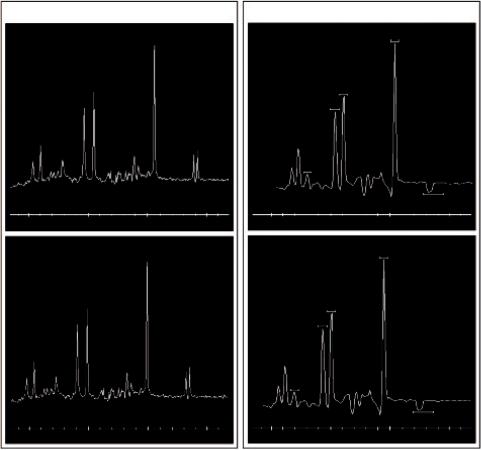
the spectrum of about 0.1 ppm to the right and needs to be corrected for in order to compare spectra. Figure 6.1 illustrates the temperature difference on a phantom measurement before and after correction.
6.2.4 Voxel Positioning
The choice of the position of the voxel is obviously of paramount importance for a meaningful in vivo 1H-MRS, as it is important to locate the voxel in the appropriate region to detect the pathology of a lesion (Drost et al., 2002). For instance, there may be necrotic or cystic areas within a brain lesion that should be avoided. Moreover, active tumor and edema should be differentiated and the voxel should be accurately positioned, first on the most informative part of the lesion (the nodular part in the case of tumors), and second on the peritumoral area (Tsougos et al., 2012). Obviously, lesions do not always place themselves in convenient positions in the brain, nor in convenient shapes. But even in the case where a lesion has an absolutely symmetrical spherical shape, it is very important to realize the potential error that might occur from the incorrect voxel placement. Figure 6.2 illustrates a case of a hypothetical, completely
|
Single Voxel |
|
|
|
|
Multivoxel |
|
|
Before temperature correction |
|
|
Before temperature correction |
|
||
|
|
|
|
|
|
NAA |
|
|
|
|
|
|
|
Cr |
|
|
|
|
|
|
Ch |
|
|
|
|
|
|
|
MI |
|
|
|
|
|
|
|
|
|
LL |
4 |
3 |
2 |
1 |
4 |
3 |
2 |
1 |
|
After temperature correction |
|
|
After temperature correction |
|
||
|
|
|
|
|
|
NAA |
|
|
|
|
|
|
Cr |
|
|
|
|
|
|
|
Ch |
|
|
|
|
|
|
|
MI |
|
|
|
|
|
|
|
|
LL |
|
4 |
3 |
2 |
1 |
4 |
3 |
2 |
1 |
FIGURE 6.1 Single voxel (left) and Multivoxel spectroscopy (right) on a standard spectroscopy phantom (25-cm-diameter MRS HD sphere; General Electric Company) at 3.0T. The frequency shift before temperature correction (upper diagrams) and after temperature correction is noticeable.
Artifacts and Pitfalls of MRS |
127 |
Vsphere = 4/3 r3 = 4.08 cm3
Vcube = a3 = 8 cm3
rrsphere = 1 cm acube = 2 cm
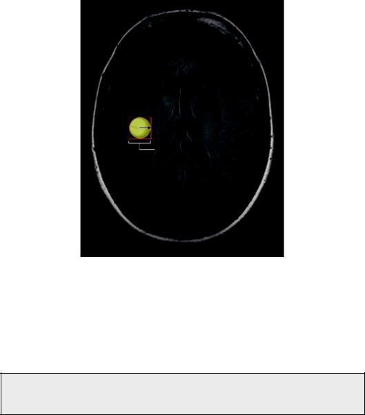
FIGURE 6.2 A case of a hypothetical, completely spherical lesion of 1 cm radius. By placing a 2 × 2 × 2 cm3 voxel, it is evident that almost half of the voxel volume will cover peritumoral area leading to approximately 50% contamination from healthy or edematous tissue.
spherical lesion of 1 cm radius. By placing a voxel or cube of a 2-cm side on the center MR axial slice as seen in Figure 6.2, one would assume the coverage is more or less appropriate. Alas, taking into account the volume of the lesion (sphere) and the volume of the voxel (cube) it is evident that almost half of the voxel volume covers an area outside the lesion.
Hence, the metabolic profile acquired would have approximately 50% contamination from healthy or edematous tissue!
Moreover, it should be realized that there is a limitation regarding the minimum voxel size that can be used to obtain adequate SNR. Small voxels are easier to shim, but the signal depends on volume; so, a voxel of 1 cm3 (1 × 1 × 1 cm) is often considered the absolute minimum size to achieve a reasonable SNR for 3T, or 3.375 cm3 (1.5 × 1.5 × 1.5 cm) the practical minimum. If one wishes to further reduce the volume of the voxel, then the number of signal averages (or number of excitations [NEX]) recorded should be substantially increased.
This of course comes with a serious penalty: a substantial increase of scan time! The SNR is approximately given by
SNR = SNR1NEX1/2VOI |
(6.2) |
128 |
Advanced MR Neuroimaging: From Theory to Clinical Practice |
where SNR1 is the SNR for a single acquisition, NEX is the number of averages (excitations), and VOI is the volume of interest, from which the spectrum is being collected. From this equation, it is evident that SNR increases more with VOI and less with NEX. Therefore, to achieve a given SNR when VOI is reduced in half, NEX should be increased at least four times! Taking into account that the acquisition time can be estimated as NEX × TR, the total examination time should be increased four times, and this might not be possible during the clinical routine.
Correct voxel localization is also beneficial when monitoring brain pathology as well as treatment effects. As mentioned earlier, in cases of heterogeneous brain tumors, within a single lesion, there may be areas of necrosis, active tumor and edema. These areas are not always distinguishable on standard T1-weighted and T2-weighted MR images but rather post-contrast (Gd) images are required to ensure correct voxel placement in the active lesion. Therefore, spectroscopic prescription should always be used for adequate positioning. Thus, the possible effects of contrast on spectroscopy need to be anticipated (please refer to the next section).
6.2.5 Use of Contrast and Positioning in MRS
The controversy regarding the reliability of 1H-MR spectroscopy findings in the presence of gadolinium chelates remains unanswered. It has been shown that gadolinium concentration has a minor effect in the signal of metabolites, causing a small amount of line broadening, so post-contrast T1 images can be useful for accurate voxel prescription (Lin and Ross, 2001; Murphy et al., 2002; Ricci et al., 2000; Taylor et al., 1995). On the other hand, this is true only if the Gd concentration of the lesion is relatively low: at higher concentrations, the T1 and T2 shortening effects should be taken into account. However, metabolite signals theoretically originate from the intracellular space where gadolinium cannot enter. Hence, the contrast agent effects reported in the literature (slight line broadening at typical, steady-state concentrations) have not been significant, although longer TEs seem to be more venerable than short TEs (Lin and Ross, 2001; Sijens et al., 1997; Sijens et al., 1998).
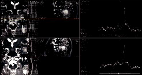
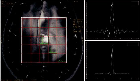
Figure 6.3 shows an example of MRS performed before and after Gd administration where post-contrast spectra are not significantly different relative to pre-contrast. The only necessary action is to readjust shimming post-Gd to account for any susceptibility differences.
FIGURE 6.3 MRS performed before and after Gd administration. Post-contrast spectra are not significantly different relative to pre-contrast.
Artifacts and Pitfalls of MRS |
129 |
Lac
ml
FIGURE 6.4 Chemical shift displacement (CSD) effect. Example of the calculated chemical shift displacement between mI and Lac at 3T. Considering all three directions, the mis-mapping can be as high as ~50%.
In conclusion, if magnetic field homogeneity can be adjusted, it appears unlikely that gadolinium can have any significant effect on brain spectra. The advent of more sophisticated medical imaging processing techniques has further improved voxel positioning within the lesion under study. Gajewicz et al. (2006) have shown that fused anatomical post-gadolinium MR imaging and single photon emission tomography (SPECT) imaging for 1H-MRS, significantly improved the diagnosis of tumor grade and type. Moreover Dou et al. (2015) investigated the possibility for automatic voxel positioning for MRS at 7T, and concluded that, in view of the highly accurate and reproducible voxel alignment with automatic voxel positioning, the application of automatic rather than manual voxel positioning in future ultrahigh-field longitudinal MRS studies could be implemented.
Last, cautious spatial localization is used to remove unwanted signals from outside the ROI, like extracranial lipids and to avoid “partial volume effects,” thereby providing a more genuine tissue characterization. Additional benefits from careful spatial voxel localization originate from the fact that variations in the main magnetic field and magnetic field gradients are greatly reduced, thereby providing narrower spectral lines and more uniform proton excitation.
6.2.6 Chemical Shift Displacement
The theoretical basis of MRS, the “chemical shift” phenomenon, can unfortunately be simultaneously the origin of an artifact called chemical shift displacement (CSD). This artifact is inherent to the use of magnetic field gradients for spatial localization via the spatial frequency dependency they create and cannot be completely avoided.
The nature of CSD artifacts between metabolites in MRS are identical to fat-water artifacts seen on conventional MRI. When a slice-selective pulse is applied, the position of the slice depends on the frequency offset and the gradient strength. The problem is that this frequency offset will be slightly different for each metabolite due to different resonance. It follows that the voxel position of each metabolite will also slightly vary, according to this difference (chemical
130 |
Advanced MR Neuroimaging: From Theory to Clinical Practice |
5 × 5
20 × 20
FIGURE 6.5 CSI multivoxel MRS technique. Voxel bleeding depends on the sampling and postprocessing scheme of the PSF (right). By increasing the number of voxels (grid size) the PSF becomes sharper, resulting in reduced voxel bleeding.
shift) and the strength of the applied gradient. At the same time, the thickness of the slice will depend on the ratio of the RF pulse bandwidth to the gradient strength. This effect will lead to metabolite contributions that originate from partially differing spatial positions.
Consider, for example, a brain voxel containing lactate (Lac) and myo-inositol (mI) as seen in Figure 6.4. Their chemical shift difference is 2.2 ppm (3.5 ppm-1.3 ppm), which according to Equation 6.1, translates into a frequency difference of about 300 Hz at 3.0T. Considering a transmit RF-bandwidth at 1.5 kHz, then the two metabolites would be spatially dispersed or mis-mapped about 20% (300/1500) relative to one another. More importantly, it has to be stressed that because this displacement would occur in all three directions, only 51% ((1−0.20)³) overlap would occur in the entire voxel, even though the two resonances should coincide exactly (Elster, MRIquestions.com). This CSD artifact not only affects the relative positions of metabolites, but also their position relative to the prescribed planning grid and hence on the relevant anatomy. Chemical shift dispersion increases linearly with magnetic field strength, therefore artifacts are most problematic at higher magnetic fields.
As mentioned earlier, this effect unfortunately cannot be avoided completely. However, it can be minimized using the highest possible bandwidth RF pulses compared to the spectral dispersion (Kaiser et al., 2008; Scheenen et al., 2008). However, specific absorption rate (SAR) limitations are a major drawback since pulses tend to require high RF power levels, and may exceed maximum values for human applications. An alternative mitigating strategy is to use high bandwidth saturation pulses since these have higher bandwidths and lower SAR than either excitation or refocusing pulses (Edden and Barker, 2007; Edden et al., 2006; Tran et al., 2000).
6.2.7 Spectral Contamination or Voxel Bleeding
Contrary to single voxel spectroscopy, the main disadvantage of multi voxel spectroscopy or CSI is the presence of the so-called spectral contamination or voxel bleeding. This effect refers to the erroneous assignment of metabolite signals and therefore contamination of a voxel from
Artifacts and Pitfalls of MRS |
131 |
adjacent locations. This artifact is due to the actual shape of the point spread function (PSF) associated with the limited spectroscopic grids (or matrix size) used, which are typically in the range of 8 × 8 to 32 × 32.
As seen in Figure 6.5, the shape of the PSF following Fourier transformation is such that the spectral peaks arising from a voxel can partially affect their neighboring voxels (spread out), although a significant truncation of the digitized signal must take place. The signal contribution (i.e., the voxel bleeding) depends on the sampling and post-processing scheme of the PSF. The exacerbation of voxel bleeding depending on low CSI grid size (matrix) is illustrated in the right part of Figure 6.5. The fewer the CSI voxels the broader the PSF, resulting in increased voxel bleeding.
This artifact cannot be completely eliminated, but it can be reduced by the use of digital filtering techniques in the spatial domain before Fourier transformation, but these result in an increase of the voxels’ dimensions. This in turn can be compensated by increasing the grid, thereby increasing the number of voxels. By increasing the number of voxels, the PSF becomes sharper resulting in reduced voxel bleeding.
Another mitigating strategy to eliminate signals outside the VOI is the application of sliceselective pulses or outer volume saturation (OVS). These pulses are used to generate suppression slices on the periphery of the VOI so as to eliminate signals from extracranial water and lipids. Especially regarding lipid contamination, this is particularly important when the investigated pathology may involve Lactate signals (indicating necrosis). To positively identify Lac, a doublet positioned at 1.3 ppm should be accurately determined. Since Lac has a longer T2 compared to lipids, it may be better to use longer rather than shorter TEs since the Lac signal will appear inverted.
6.2.8 To Quantify or Not to Quantify?
Generally, there is a dispute in the MRS community regarding the issue of quantification versus visual interpretation and metabolite ratio evaluation. Obviously, the ultimate goal of MRS data analysis is to accurately determine metabolite concentrations based on the proportionality of metabolite resonance peak areas. Quantitative analyses of the (spectral) data, as well as the methods for this analysis arguably have the same importance as the techniques used to collect them. Possible incorrect data analysis or potential artifacts and pitfalls may lead to systematic errors and hence misinterpretation of the clinical results.
There can be different approaches regarding the quantification of spectra, and these can be broadly distinguished into the “relative” versus “absolute” quantification techniques.
6.2.8.1 Relative Quantification
The most widely used method of relative quantification is the use of an internal or endogenous metabolite, which can be used as the reference metabolite value. With this approach, each metabolite of interest in a given spectrum is normalized to the signal value of total Creatine (tCr - creatine plus phosphocreatine), which is commonly used as the reference metabolite since it is a strong signal with relatively low variability across brain regions and across subjects.
This technique is also called normalization (or “creatine normalization”) because it reduces the variance due to the unknown scaling factor (see Section 6.2.2) in a given spectrum. That is, in any given acquisition, the different scaling factor would influence all metabolite signals equally; hence, any difference would cancel out when ratios are used. Obviously, these “metabolite ratios” do not reflect true concentrations unless the concentration of the reference metabolite is known.
Moreover, normalization removes another potential systematic error: the partial volume effect from the cerebrospinal fluid (CSF). Hence, although not absolute, normalization is still
132 |
Advanced MR Neuroimaging: From Theory to Clinical Practice |
considered by many investigators the most robust, safe, and reproducible of all MRS quantitation techniques since it does not require extra time, software, or sequence modifications, and can be considered a reliable marker of tissue biochemistry. Nevertheless, the aforementioned normalization is only valid under the assumption that total creatine concentration does not vary across regions and subjects, which unfortunately is not the case. This variation across subjects is generally random, with a range of no more than 10%–15% (Webb et al., 1994) and is expected to decrease when many creatine-normalized metabolites are compared across different groups of patients.
Furthermore, relative quantification is associated with one more pitfall: the fact that an abnormal ratio might be equally the result of a change in the numerator, the denominator or even both, and therefore, ratios are intrinsically ambiguous and prone to systematic errors. For example, a reduced NAA/Cr ratio in the brain is interpreted as decreased NAA concentration, and therefore, associated with neuronal loss; however, a reduced NAA/Cr ratio may also be a result of increased Cr, which has been observed for instance in multiple sclerosis (Inglese et al., 2003).
6.2.8.2 Absolute Quantification
In order to resolve the uncertainties associated with the use of metabolite ratios, a variety of absolute quantification techniques have been devised.
6.2.8.2.1 Use of Water as an Internal Reference Signal
Since the water content in the brain tissue is almost constant, an alternative and widely used method for measuring metabolite concentrations is the use of unsupressed tissue water signal as an internal reference (De Graaf, 2007; Ernst et al., 1993; Malucelli et al., 2009). Brain water content is well known and can be evaluated relatively easily by turning off the water suppression pulses (Christiansen et al., 1993; Thulborn and Ackerman, 1983). Moreover, comparing the water signal to creatine signal, the pathology-associated changes are relatively small. More specifically, the water content in gray and white matter varies about 10% (from 70% to 80%), and it is estimated that the proton concentration in the brain parenchyma is of the order of 77–88 M (M = molarity = mol/L). As in the case of creatine, the internal reference technique of water has the advantage of eliminating many potential systematic errors and pitfalls since it is acquired from the same VOI, with same sequence parameters, hence the metabolite concentration estimation becomes relatively accurate. Nevertheless, it must be noted that an additional structural MR image of the tissue within the voxel must be acquired to differentiate gray and white matter, and CSF, so that after coregistration, a segmentation of the voxel will follow (Gussew et al., 2012).
Obviously, there are several associated limitations and the use of water as an internal reference signal may be more complex than it appears. First, we have the basic assumption of the water content. This assumption is of course prone to error, particularly in unknown diseases and within focal lesions (Kreis, 2012). The differences in the water content of gray and white matter can be taken into account with segmentation information as already mentioned, but there is also the error due to unexpectedly high water contributions from CSF or cysts that may be included in the VOI due to the relatively large MRS voxels used (a practical minimum is of the order of 3.375 cm3 at 3T). Also, brain water content may be variable in several cases, like in neonatal studies, or heterogeneous pathologies involving major changes in brain tissue.
6.2.8.2.2 Absolute Concentrations Using External Reference
Absolute concentrations using external reference involve the placement of a reference vial containing a known concentration, in a region outside the primary area of interest (e.g., next

Artifacts and Pitfalls of MRS |
133 |
to the head) within the coil, simultaneously with the patient. The MR signal from this reference vial is measured, either before or after the brain spectrum is recorded, but, in any case, while the patient is still in the coil to ensure the same measurement condition, like loading and RF calibration. This way, the reference concentration is exactly known, allowing the measurement of the metabolite concentrations as well as the water content of the human brain with great precision. The disadvantage is that, because the reference vial is situated at a different spatial region compared to the MRS voxel, the reference signal intensity will be affected by inhomogeneities in the RF field. Another drawback of this technique is that the presence of the external vial may degrade the B0 field homogeneity within the brain due to magnetic susceptibility effects and is also susceptible to variations of the RF field. Last, some additional time is required for the second scan increasing the overall acquisition time.
6.2.8.2.3 Absolute Concentrations Using a Phantom
The use of a phantom or the “phantom replacement” technique is a variation of the external reference technique. It involves the acquisition of a spectrum from a phantom (comparable in size to a human head) of a reference metabolite of known concentration (e.g., creatine) before or after the patient has been imaged. In other words, the phantom replaces the head of the patient and the MRS scan is repeated with identical conditions. The advantage of this technique is that the voxel can be located at exactly the same position as in the patient (with respect to the coil) providing the same scaling factor, which can be calculated from the ratio of the metabolite peak integral with the known metabolite concentration in the phantom (Buonocore and Maddock, 2015). Obviously, various correction factors have to be applied; especially corrections taking into account the differences in RF coil loading that occur between the patient and the phantom since the main magnetic field should be re-shimmed to produce optimum spectra. One way of determining the loading factor is from the amount of RF power needed for a reference 90° pulse (Michaelis et al., 1993) or water suppression pulse (Danielsen and Henriksen, 1994). Finally, the extra time here is not an issue since it does not involve the patient. Summarizing all the aforementioned, Table 6.1 depicts the outline of all available MRS quantitation methods, listing their relative advantages and disadvantages.
TABLE 6.1 Summary of All Available MRS Quantitation Methods, Listing Their Relative Advantages and Disadvantages
Method |
Advantages |
Disadvantages |
|
|
|
“Metabolite ratios” |
Simple, no additional scan time, |
Cannot quantify metabolite concentrations, |
|
systematic errors, reproducible |
pathological and regional variations of |
|
|
reference metabolite common |
Spectrum from |
Normative data from subject, |
Extra scan time required, sensitive to motion |
contralateral area |
simple, no coil loading errors |
errors, not applicable in diffuse diseases, or |
|
|
midline structures |
Internal water |
Minimal extra scan time, |
Can be affected by pathological conditions |
|
simple, robust |
|
External reference |
Accurate reference |
Extra scan time required, complicated due to |
|
concentration |
susceptibility effects, B1 errors possible |
Phantom |
No extra patient scan time |
RF coil loading correction required |
replacement |
required, accurate reference |
|
|
concentration, reduced |
|
|
susceptibility effects |
|
|
|
|
134 |
Advanced MR Neuroimaging: From Theory to Clinical Practice |
6.2.9 Available Software Packages for Quantification and Analysis of MRS Data
A variety of software packages for the quantification and analysis of MRS data are available. In the following section, a brief informative description of the most commonly used packages is included so that the interested reader can proceed to a more comprehensive analysis, evaluation, and comparison. Most of these software packages are freely available, excluding the LCModel.
6.2.9.1 LCModel
One of the first software packages developed for MR automatic quantification of in vivo proton MR spectra and one of the most commonly used spectrum fitting tools is the so-called LCModel. It was established about 25 years ago (Provencher, 1993), and it was named after the analysis procedure it follows as a linear combination of model (LCModel) spectra, or basis spectra (Provencher, 2001). An example of an LCModel test run fit output is shown in Figure 6.6. The original data are shown in black, and the results of the LCModel fit in red with the metabolite ratios over Cr with their standard deviations on the right.
The advantage of the LCModel is that it is highly automated, requiring minimum user input compared to other software, especially in interdepartmental studies, where user dependency can be a major drawback for sound interpretations. Unfortunately, this is not freely available software and requires the purchase of a license, although there is a discount for nonprofit organizations. Nevertheless, it is the most widely used program, in part because of its commercial availability but also because phase, frequency and baseline correction is included in an almost fully automated procedure. Another important advantage of LCModel is the automatic
FIGURE 6.6 Example of the LCModel fit output. (Adapted from software’s webpage: http://s- provencher.com/lcmodel.shtml.)
Artifacts and Pitfalls of MRS |
135 |
preprocessing of spectra, including built-in corrections for eddy current artifacts, which almost eliminates phase and fitting errors that might result from incorrect user parameter adjustments.
Generally, in order to improve fitting results, basis metabolite sets should be included in the system. These can be provided by the software vendor, although user generated basis sets, including macromolecules, is a safer and more robust choice. The fitting in LCModel is performed in the frequency and not in the time domain as in other software, with a data-based lineshape function, which theoretically takes into account different experimental conditions as it is nearly model-free. Another advantage of LCModel regarding CSI data analyses is that it first analyzes a central voxel of the subset and then works outwards, using Bayesian learning to get starting estimates and “soft constraints” for the first-order phase correction and the referencing shift from the preceding (often better) central voxels for the (often poorer) outer voxels. This speeds up and improves the overall analyses. LCModel is compatible with the majority of clinical MRS data formats.
6.2.9.2 jMRUI
jMRUI is a software package for advanced analysis of MRS and spectroscopic imaging (MRSI) data. The analysis is performed in the time-domain using signal processing algorithms to analyze and quantify spectroscopic data: from a single spectrum to a full multidimensional MRSI dataset (Naressi, 2001; Naressi et al., 2001; Stefan et al., 2009). The time domain is selected in order to limit data imperfections (signal truncation, echo timing errors, and spectral baseline) arising from FFT-processed data, with fewer assumptions and approximations.
The software interfaces algorithms for frequency selective filtering of signals, including both peak fitting and basis spectrum fitting (e.g., removal of residual water), correction of eddycurrent artifacts, linear prediction, non-linear fitting (quantitation of metabolites), and many more.
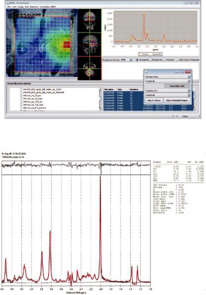
The basic algorithm for basis spectra fitting is quantitation based on quantum estimation (QUEST) (Ratiney et al., 2004; Ratiney et al., 2005), and for peak fitting, one of the most commonly used peak fitting software packages for in vivo MRS, called AMARES (advanced method for accurate, robust, and efficient spectral fitting) (Vanhamme et al., 1997). QUEST fits the spectral data to a basis set in the time domain in a number of ways (e.g., truncation, FID weighting), while AMARES is based on a great wealth of prior knowledge constraints. Nevertheless, the entire spectral analysis can be performed using a set of mathematical model state-space fitting methods, using limited or even no prior knowledge. jMRUI is proprietary software distributed under its own license terms, and made freely available to registered users for non-commercial use. An example of the Cho/Cr metabolite map in a GBM-patient brain with jMRUI is illustrated in Figure 6.7.
Web Link: jMRUI, http://www.mrui.uab.es/mrui/mrui_Overview.shtml
6.2.9.3 TARQUIN
TARQUIN (totally automatic robust quantitation in NMR) is a freely distributed analysis tool for automatically determining the quantities of molecules present in in-vivo 1H MRS and exvivo with 1H HR-MAS spectroscopy data. The intended purpose of TARQUIN is to aid the characterization of pathologies, in particular brain tumors, based on a flexible time-domain fitting routine designed to give accurate, rapid and automated quantitation for routine analysis (Wilson et al., 2011). It includes a quantum mechanically based metabolite simulator to allow basis set construction optimized for the investigation of particular pathologies’ sequence parameters. One unique feature included in TARQUIN is that it offers the possibility of
136 |
Advanced MR Neuroimaging: From Theory to Clinical Practice |
FIGURE 6.7 New jMRUI clinical viewer plug-in for MRS and MRSI: Cho/Cr metabolite map in a GBMpatient brain. (Adapted from software’s webpage: http://www.mrui.uab.es/mrui/mrui_Overview.shtml.)
FIGURE 6.8 Example fit to the braino phantom (1.5T, PRESS TE = 30 ms) in TARQUIN. (Adapted from software’s webpage: http://tarquin.sourceforge.net/.)
applying soft constrains on the metabolite peaks based on prior knowledge of relative concentrations for more accurate estimations. Moreover, it is compatible with most clinical MRS data in the standard DICOM format. An example fit to the braino phantom (1.5T, PRESS TE = 30 ms) is illustrated in Figure 6.8. Web Link: TARQUIN, http://tarquin.sourceforge.net/.
6.2.9.4 SIVIC
SIVIC is an open-source, standards-based software framework and application suite for processing and visualization of DICOM MRS data. It enables a complete scanner-to-PACS
Artifacts and Pitfalls of MRS |
137 |
workflow for evaluation and interpretation of MRSI data. One unique feature of SIVIC is that it supports conversion of vendor-specific formats into the DICOM MR spectroscopy (MRS) standard, providing modular and extensible reconstruction and analysis pipelines, and tools to support visualization requirements associated with such data (Crane et al., 2013).
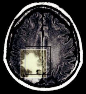
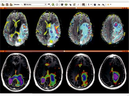
The benefit is that the entire exam including MRSI data and derived 3D metabolite maps can be archived in PACS. A key point here is that these 3D DICOM data are available for evaluation with any 3D imaging data in a multimodal evaluation scheme. An example is given in Figure 6.9, where the metabolite maps (bottom color overlay on a T1 contrast enhanced image) derived from MRSI data in SIVIC are exported as standard DICOM MR Image Storage SOP instances, which can be loaded into 3D DICOM image analysis software packages (shown here in 3D Slicer). The top panel shows ADC maps (color) on FLAIR images. SIVIC, http://sourceforge.net/projects/sivic/.
6.2.9.5 AQSES
AQSES (Automated Quantitation of Short Echo-time MRS Spectra) is a software package for quantitation of short echo time magnetic resonance spectra only, developed in JAVA (Poullet et al., 2007). The quantitation is approached in the time domain using the nonlinear least squares fitting, with a variable projection procedure. AQSES includes several preprocessing methods like phase-, frequencyand eddy current correction. Moreover, it includes a max- imum-phase FIR filter or the HLSVD-PRO filter to remove unwanted components such as residual water. A macromolecular baseline is incorporated into the fit via nonparametric modeling, with penalized splines. This attribute can be viewed as a possible limitation since there is no prior knowledge of the macromolecule signals. Nevertheless, a graphical user interface for optimized quantitation is included and is therefore very suitable for spectroscopic imaging data. AQSES is freely available online from http://homes.esat.kuleuven.be/~biomed/software
.php under an open source license.
FIGURE 6.9 Example output from the SIVIC software. (Courtesy of Jason Crane, UCSF.)

138 |
Advanced MR Neuroimaging: From Theory to Clinical Practice |
6.3 Conclusion
Based on an extended review of the literature as well as personal clinical experience with 3T MR spectroscopy for the last 10 years, it is safe to argue that MRS can significantly improve the overall diagnostic accuracy of brain MRI, leading to safer and more robust clinical decisions, improving the efficiency of patient management. My personal opinion is that MRS should be integrated into a multi-parameter multi-modality approach of brain diseases for improved quantification accuracy.
Nevertheless, there should be an even greater degree of attention to the data analysis methods and new acquisition protocols used since the improved and advanced processing techniques also have the potential to optimize the clinical application of MRS. In spite of the deficiencies and potential artifacts and pitfalls of clinical MRS, it has proven to be a very powerful technique for the dynamic monitoring of brain tumor metabolism, and the progress in technology in the next few years is expected to increase the technique’s application efficiency.
References
Buonocore, M. H. and Maddock, R. J. (2015). Magnetic resonance spectroscopy of the brain: A review of physical principles and technical methods. Reviews in the Neurosciences, 26(6), 609–632. doi:10.1515/revneuro-2015-0010
Christiansen, P., Henriksen, O., Stubgaard, M., Gideon, P., and Larsson, H. (1993). In vivo quantification of brain metabolites by 1H-MRS using water as an internal standard. Magnetic Resonance Imaging, 11(1), 107–118. doi:10.1016/0730-725x(93)90418-d
Crane, J. C., Olson, M. P., and Nelson, S. J. (2013). SIVIC: Open-source, standards-based software for DICOM MR spectroscopy workflows. International Journal of Biomedical Imaging, 2013, 1–12. doi:10.1155/2013/169526
Danielsen, E. R. and Henriksen, O. (1994). Absolute quantitative proton NMR spectroscopy based on the amplitude of the local water suppression pulse. Quantification of brain water and metabolites. NMR in Biomedicine, 7(7), 311–318. doi:10.1002/nbm.1940070704
De Graaf, R. A. (2007). In Vivo NMR Spectroscopy Principles and Techniques. Chichester, UK: Wiley.
Dou, W., Benner, T., Kaufmann, J., Li, M., Speck, O., Walter, M., and Zhong, K. (2015). Automatic voxel positioning for MRS at 7 T. MAGMA, 28(3), 259–270.
Drost, D. J., Clarke, G. D., and Riddle, W. R. (2002). Proton magnetic resonance spectroscopy in the brain: Report of AAPM MR Task Group #9. Medical Physics, 29(9), 2177–2197.
Ebel, A. and Maudsley, A. A. (2005). Detection and correction of frequency instabilities for volumetric 1H echo-planar spectroscopic imaging. Magnetic Resonance in Medicine, 53(2), 465–469. doi:10.1002/mrm.20367
Edden, R. A. and Barker, P. B. (2007). Spatial effects in the detection of γ-aminobutyric acid: Improved sensitivity at high fields using inner volume saturation. Magnetic Resonance in Medicine, 58(6), 1276–1282. doi:10.1002/mrm.21383
Edden, R. A., Schär, M., Hillis, A. E., and Barker, P. B. (2006). Optimized detection of lactate at high fields using inner volume saturation. Magnetic Resonance in Medicine, 56(4), 912–917. doi:10.1002/mrm.21030
Elster, A. D. (2017). MRI questions and answers. MR Imaging Physics and Technology, http:// www.mriquestions.com/.
Ernst, T., Kreis, R., and Ross, B. (1993). Absolute quantitation of water and metabolites in the human brain. I. Compartments and water. Journal of Magnetic Resonance, Series B, 102(1), 1–8. doi:10.1006/jmrb.1993.1055
Artifacts and Pitfalls of MRS |
139 |
Gajewicz, W., Grzelak, P., Gorska-Chrzastek, M., Zawirski, M., Kusmierek, J., and Stefanczyk, L. (2006). The usefulness of fused MRI and SPECT images for the voxel positioning in proton magnetic resonance spectroscopy and planning the biopsy of brain tumors: Presentation of the method. Neurologia i Neurochirurgia Polska, 40, 284–290.
Gussew, A., Erdtel, M., Hiepe, P., Rzanny, R., and Reichenbach, J. R. (2012). Absolute quantitation of brain metabolites with respect to heterogeneous tissue compositions in 1H-MR spectroscopic volumes. Magnetic Resonance Materials in Physics, Biology and Medicine,
25(5), 321–333. doi:10.1007/s10334-012-0305-z
Hoult, D. I. and Richards, R. E. (2011). The signal-to-noise ratio of the nuclear magnetic resonance experiment. 1976. Journal of Magnetic Resonance, 213(2), 329–343.
Inglese, M., Li, B. S., Rusinek, H., Babb, J. S., Grossman, R. I., and Gonen, O. (2003). Diffusely elevated cerebral choline and creatine in relapsing-remitting multiple sclerosis. Magnetic Resonance in Medicine, 50(1), 190–195. doi:10.1002/mrm.10481
Kaiser, L. G., Matson, G. B., and Young, K. (2008). Numerical simulations of localized high field 1H MR spectroscopy. Journal of Magnetic Resonance, 195(1), 67–75.
Kreis, R. (2012). Clinical MRS: Promise, Potential, Power and Pitfalls. Proceedings of the International Society for Magnetic Resonance in Medicine, 20.
Lin, A. P. and Ross, B. D. (2001). Short-echo time proton MR spectroscopy in the presence of gadolinium. Journal of Computer Assisted Tomography, 25(5), 705–712. doi:10.1097/00004728-200109000-00007
Malucelli, E., Manners, D. N., Testa, C., Tonon, C., Lodi, R., Barbiroli, B., and Iotti, S. (2009). Pitfalls and advantages of different strategies for the absolute quantification of N-acetyl aspartate, creatine and choline in white and grey matter by 1H-MRS. NMR in Biomedicine, 22, 1003–1013. doi:10.1002/nbm.1402
Michaelis, T., Merboldt, K. D., Bruhn, H., Hänicke, W., and Frahm, J. (1993). Absolute concentrations of metabolites in the adult human brain in vivo: Quantification of localized proton MR spectra. Radiology, 187(1), 219–227. doi:10.1148/radiology.187.1.8451417
Murphy, P. S., Dzik-Jurasz, A. S., Leach, M. O., and Rowland, I. J. (2002). The effect of Gd-DTPA on T1-weighted choline signal in human brain tumours. Magnetic Resonance Imaging, 20(1), 127–130. doi:10.1016/s0730-725x(02)00485-x
Naressi, A. (2001). Java-based graphical user interface for the MRUI quantitation package. Magnetic Resonance Materials in Biology, Physics, and Medicine, 12(2–3), 141–152. doi:10.1016/s1352-8661(01)00111-9
Naressi, A., Couturier, C., Castang, I., Beer, R. D., and Graveron-Demilly, D. (2001). Java-based graphical user interface for MRUI, a software package for quantitation of in vivo/medical magnetic resonance spectroscopy signals. Computers in Biology and Medicine, 31(4), 269–286. doi:10.1016/s0010-4825(01)00006-3
Poullet, J., Sima, D. M., Simonetti, A. W., Neuter, B. D., Vanhamme, L., Lemmerling, P., and Huffel, S. V. (2007). An automated quantitation of short echo time MRS spectra in an open source software environment: AQSES. NMR in Biomedicine, 20(5), 493–504. doi:10.1002/nbm.1112
Provencher, S. W. (1993). Estimation of metabolite concentrations from localized in vivo proton NMR spectra. Magnetic Resonance in Medicine, 30(6), 672–679. doi:10.1002/ mrm.1910300604
Provencher, S. W. (2001). Automatic quantitation of localized in vivo 1H spectra with LCModel.
NMR in Biomedicine, 14(4), 260–264.
Ratiney, H., Coenradie, Y., Cavassila, S., Ormondt, D. V., and Graveron-Demilly, D. (2004). Time-domain quantitation of 1 H short echo-time signals: Background accommodation.
MAGMA Magnetic Resonance Materials in Physics, Biology and Medicine, 16(6), 284–296. doi:10.1007/s10334-004-0037-9
140 |
Advanced MR Neuroimaging: From Theory to Clinical Practice |
Ratiney, H., Sdika, M., Coenradie, Y., Cavassila, S., Ormondt, D. V., and Graveron-Demilly, D. (2005). Time-domain semi-parametric estimation based on a metabolite basis set. NMR in Biomedicine, 18(1), 1–13. doi:10.1002/nbm.895
Ricci, P. E., Coons, S. W., Heiserman, J. E., Keller, P. J., and Pitt, A. (2000). Effect of voxel position on single-voxel MR spectroscopy findings. AJNR. American Journal of Neuroradiology, 21(2), 367–374.
Scheenen, T. W., Heerschap, A., Klomp, D. W., and Wijnen, J. P. (2008). Short echo time 1H-MRSI of the human brain at 3T with minimal chemical shift displacement errors using adiabatic refocusing pulses. Magnetic Resonance in Medicine, 59(1), 1–6.
Sijens, P. E., Bent, M. J., Dijk, P. V., Nowak, P. J., and Oudkerk, M. (1997). 1H chemical shift imaging reveals loss of brain tumor choline signal after administration of Gd-contrast.
Magnetic Resonance in Medicine, 37(2), 222–225.
Sijens, P. E., Dijk, P. V., Levendag, P. C., Oudkerk, M. and Vecht, C. J. (1998). 1H MR spectroscopy monitoring of changes in choline peak area and line shape after Gd-contrast administration. Magnetic Resonance Imaging, 16(10), 1273–1280.
Taylor, J. S., Reddick, W. E., Kingsley, P. B., and Ogg, R. J. (1995). Proton MRS after gadolinium contrast agent. Third Scientific Meeting and Exhibition of the Society of Magnetic Resonance, In: Proceedings of the Society of Magnetic Resonance, Nice, France.
Thiel, T., Czisch, M., Elbel, G. K., and Hennig, J. (2002). Phase coherent averaging in magnetic resonance spectroscopy using interleaved navigator scans: Compensation of motion artifacts and magnetic field instabilities. Magnetic Resonance in Medicine, 47(6), 1077–1082. doi:10.1002/mrm.10174
Thulborn, K. R. and Ackerman, J. J. (1983). Absolute molar concentrations by NMR in inhomogeneous B1. A scheme for analysis of in vivo metabolites. Journal of Magnetic Resonance (1969), 55(3), 357–371. doi:10.1016/0022-2364(83)90118-x
Tofts, P. (2003). Quantitative MRI of the Brain: Measuring Changes Caused by Disease. Chichester, UK: John Wiley & Sons.
Tran, T. C., Vigneron, D. B., Sailasuta, N., Tropp, J., Roux, P. L., Kurhanewicz, J., and Hurd, R. (2000). Very selective suppression pulses for clinical MRSI studies of brain and prostate cancer. Magnetic Resonance in Medicine, 43(1), 23–33. doi:10.1002/ (sici)1522-2594(200001)43:1<23::aid-mrm4>3.0.co;2-e
Vanhamme, L., Boogaart, A. V., and Huffel, S. V. (1997). Improved method for accurate and efficient quantification of MRS data with use of prior knowledge. Journal of Magnetic Resonance, 129(1), 35–43. doi:10.1006/jmre.1997.1244
Webb, P. G., Sailasuta, N., Kohler, S. J., Raidy, T., Moats, R. A., and Hurd, R. (1994). Automated single-voxel proton MRS: Technical development and multisite verification. Magnetic Resonance in Medicine, 31(4), 365–373. doi:10.1002/mrm.1910310404
Wilson, M., Reynolds, G., Kauppinen, R. A., Arvanitis, T. N., and Peet, A. C. (2011). A constrained least-squares approach to the automated quantitation of in vivo 1H magnetic resonance spectroscopy data. Magnetic Resonance in Medicine, 65(1), 1–12. doi:10.1002/ mrm.22579