01 POWER ISLAND / 02 H2+NH3 / Royal Swiss 2024 Techno-Economic Analysis of Wind Power-to-Hydrogen

CHAPTER 4. GÄVLE HARBOR

Gävle harbor is the largest logistics hub in mid Sweden, where six million tons of goods are annually handled. Its infrastructure consists of six different terminals, including bulk, container, energy, and combined terminal. These terminals are managed by various specialized companies and are daily visited by large transport ships and trains. The operations taking place in the harbor include, among other things, the export of the region’s industrial production of steel, wood, and paper, while simultaneously importing raw materials for industry, consumer products, fuel, and project cargoes [75].

Gävle harbor has the aim to contribute to the global transition process of implementing green operating methods. Specifically, the Gävle harbor has planned to execute a 10-year program called “Energy-Optimized Port Cluster 2030”, where the main mission is to reduce CO2-emissions and promote energy efficiency, both at national and regional level in accordance with the Paris Agreement [75]. This program includes the entire operations taking place in the port, and therefore will be carried out in a collaboration with the companies present in the port. Some of the actions that will take place in the program are [75]:

Sustainable development of the port – implementing methods that yield in enhanced energy efficiency and increase the usage of electrically powered vehicles.

Electrify the railways that are directly connected to the terminals – infrastructure investment by the Swedish Transport Agency.

Sustainable cargo management – the container terminal’s cranes will either be operating on fossil-free fuels such as green hydrogen or electrified.

Green transportation – the use of green fuels when transporting goods from the

region’s industries to the port. The aim is to reduce CO2-emissions from the heavy truck traffic.

Furthermore, Gävle harbor AB is also actively engaging in the development of regional hydrogen infrastructure. The port has planned to dedicate a “green refueling zone”, where fossil-free fueled operating trucks can visit and refill the tank [75]. As previously mentioned, the company Svea Vind Offshore is currently in the process of developing a grid-powered hydrogen production facility in the harbor. In the future, this company also plans to construct an offshore wind plant right outside of the harbor, and Mattias Wärn, CEO of Svea Vind Offshore, in an article says that from the perspective of hydrogen production, this could mean a significant increase in production scale [76].

4.1 Vehicles Operating in Gävle Harbor

This section aims to provide an insight into the various types of vehicles operating in the port, and the methodology employed to estimate the respective diesel consumption. The purpose is to apply equation (10) to calculate the corresponding hydrogen consumption. Based on this, information about the harbor’s hypothetical daily hydrogen demand can be computed.

49

4.1.1 Trucks

The haulage contractors in the harbor, have reported that an average of 202 specific trucks are operating in the port every day, where each is estimated to consume about 230 l diesel/day. This information can be used to determine the corresponding hydrogen consumption by applying equation (10), with the specific variable’s values listed in Table 25. The calculated corresponding hydrogen consumption of these trucks is available in Appendix E, Table 58.

Table 25. Data of diesel engine, Fuel cell, and the corresponding fuels [19].

4.1.2 Machines

The loading machines operating in the harbor are majority owned by Yilport, while some belongs to Sören Thyr AB. The quantity and types of machines operating in the terminals are listed in Table 26 [19].

Table 26. Specific Data and Information Regarding the Machines Operating in Gävle Habor [19].

In contrast to the calculation of the trucks’ hydrogen consumption, some of the assumptions about the machines needs to be made prior to calculation of the diesel consumption. This includes considering which type of fuel is being used due to some machines are HVO-fueled. In this report, it is assumed that all machines are operating on diesel fuel. Furthermore, certain machines in the harbor, such as small forklifts, are already electrically powered. However, the number of electrified forklifts in the port are unavailable. This means that the actual number of forklifts needing a transition to green fuel is lower than what is specified in Table 26. The sizes of Sören Thyr AB’s machines were unknown, therefore, these machines will henceforth be assumed to have the similar sizes as Yilport’s machines [19].

Technical information about the machines were limited, due to some manufacturers being unknown and therefore assumptions were made. The manufacturer Kalmar’s product catalogue was used as a reference to estimate the diesel consumption of reachstackers and forklifts (lift capacity larger than 5 tons) [19]. This is due to around 35% of Yilport’s machines were from the manufacturer Kalmar. The performance data of the reachstackers in the Kalmar catalogue were

50

presented in ranges, where the mean value was used to compute the diesel consumption. Apart from the manufacturer Kalmar, technical information could also be obtained from manufacturer Linde as 13% of Yilport’s machines were from there. This information was used to compute the diesel consumption of forklifts with a lift capacity of lower than 5 tons [19].

The diesel-fueled Kalmar machines are equipped with diesel engines that were manufactured by Volvo. The engine efficiency can be estimated to be around 50% [19]. This value was assumed in all calculations of hydrogen consumption when implementing equation (10). Technical data about the diesel and corresponding hydrogen consumption for the forklifts and reachstackers, are available in Appendix D, Table 59 and 60, respectively [19].

Moreover, estimation of the wheel loaders’ diesel consumption required additional assumptions in terms of the drivers’ operating behavior. That is the diesel consumption of such vehicles were directly influenced by how these vehicles were operated by the driver [19]. Technical information regarding the diesel consumption of the wheel loaders were obtained from [19], which provided data about various models’ fuel consumption based on different workloads (low, medium, or high). In this report, the wheel loaders were assumed to operate at a medium load. The diesel consumption and the corresponding hydrogen consumption of the wheel loaders could be calculated and are available in Table 61, in Appendix E [19].

Technical information about the terminal tractors were obtained from [19]. According to this source, terminal tractors were estimated to consume about 4.55 l diesel/h. This value was applied to the terminal tractor of Gävle harbor, and the computed hydrogen consumption is listed in Table 62 [19]. To estimate the daily hydrogen consumption of these machines, it was assumed that a standard working day in the harbor consist of 8 hours for a whole year (365 days).

4.1.3 Transition Process

The transition process from diesel fueled to green hydrogen fueled vehicles is expected to occur gradually. Therefore, three different hydrogen transition stages are proposed: 15%, 50% and 100% of the daily hydrogen demand required to operate the trucks and machines of the Gävle harbor. The final stage represents a fully green-fueled operating harbor, where the PtH plant is capable to provide 100% of the daily hydrogen demand. Furthermore, these transition stages will serve as a foundation to estimate within which range the hydrogen produced from the three different facility sizes, would fall within. The daily hydrogen demand of the respective transition stage is presented in Table 27. This table is based on the vehicle composition listed in Table 63, in Appendix E.

Table 27. Daily hydrogen demand based on transition stages [19].

51

generated from the sales of electricity and electricity certificate. These are expressed in equations 14 and 15, respectively.

The total generated income can be obtained by subtracting (14) from (15) as seen in equation 16.

WG3 in equation (16) is the alternative income obtained if the electricity would have been sold to the grid instead of powering the hydrogen production facility. Therefore, equation (16) will be integrated into the calculations of the break-even spot prices in equation (30), as the opportunity cost.

5.1.2 Hydrogen Production Facility

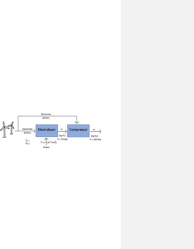
In this section, the operational processes of the main equipment are derived from the flowchart visualized in Figure 23 and expressed in the form of operational equations as described in section 5.1.2.1–5.1.2.3. The operational equations for each unit are then converted into variable cost equations. Moreover, in the hydrogen production simulation, factors such as the spot price, target year, generated wind power and electrolyzer capacity, are considered. The Python code utilized to simulate the H2 production is available in Appendix B.

Figure 23. A simplified flowchart of the H2 production facility’s operational process.

5.1.2.1 Variable Operational Process of Electrolyzer

In this thesis, the variable operation (VOElec) for all electrolyzer units includes the following two

two parameters; power (Epower) (MWh/kg H2) and water (Wcons) (kg H2O(l)/kg H2) consumptions. This is due to electricity and water being the only feedstocks to the water electrolyzer as seen in Figure 23. The operational cost of an electrolyzer can be obtained by linking its consumption cost

of power (Epower) (MWh/kg H2) and water (Wcons) (kg H2O(l)/kg H2) to the spot price (€/MWh) and water cost (CW) (€/kg H2O), respectively. However, since this report involves operating the hydrogen production site at profitable production hours, the power consumption of electrolyzer

(Epower) (MWh/kg H2) will be linked to equation (16) as expressed in the equations (18) and (19). This is due to the aim of finding spot prices where it is more profitable to produce hydrogen over selling the electricity to the grid.

53

Table 32. Parameters of Annuity Method [80].

57