Fig. 10.1 Relationships between tree height and aboveground biomass for several boreal forest

species in interior Alaska, USA [57]. Line shows the predicted values from the regression model, m = ah2

10.2 Aerial Photo Mensuration

In this section, we firstly describe the principles of aerial photogrammetry and then we go on to describe how this is used to form tree height measurements.

10.2.1 Principles of Aerial Photogrammetry

Aerial photogrammetry,1 or the science of making measurements from aerial photographs, has been used to support forestry applications for well over half a century

1It should be noted that the terminology describing identical geometric principles and analytical procedures often differs between the fields of photogrammetry and computer vision. For the purposes of clarity, the following table denotes the photogrammetry terminology and the corresponding computer vision terms:

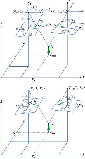
[43, 51]. Furthermore, aerial photo mensuration, or forest photogrammetry, is the science of acquiring forest measurements from aerial photographs [40]. As mentioned above, tree height is one of the most fundamental measurements in forest inventory and the use of aerial photogrammetry to collect accurate and precise tree height measurements from a remote platform is a primary goal of aerial photo mensuration. Although there are several methods used to acquire tree height information from aerial photos, the most reliable method of tree height measurement, if also the most complex and difficult to carry out in practice, is based on the measurement of stereo disparity on overlapping pairs of aerial photographs (see Fig. 10.2). From a mathematical standpoint, the measurement of tree heights within the overlap area of a stereo pair is carried out by taking the distance between the elevation measured at the base of the tree (Xp , Yp , Zbase) and the elevation measured at the top of the tree (Xp , Yp , Zp ) (see Fig. 10.2). Once the exact position and orientation of each photo in the stereo pair is determined (using ground control points and a procedure known as exterior orientation), then these elevations can be determined using the collinearity condition, which states that the ray from the optical center to the image feature and the ray from the optical center to the corresponding world feature are collinear. Given that two collinearities are formed on the same scene point, we can intersect them to determine the 3D location of the scene point (see Fig. 10.2) [56].

10.2.1.1 Geometric Basis of Photogrammetric Measurement

In mathematical terms, the collinearity condition for a feature on the ground (P) that is seen at point (p1) in image 1 (Fig. 10.2) is expressed by the so-called collinearity equations, based on the geometric principle that the ray from the optical center to the image feature and the ray from the optical center to the corresponding real world feature are collinear [56]:

Here the elements of the rotation matrix M = {mij }3i,j,3=1,1 are functions of the rotation angles (κ , ϕ, ω) that define the orientation of camera for each exposure:

Fig. 10.2 Geometric basis for measurement of tree heights using the collinearity principle and space forward intersection from a stereo pair of aerial photographs. For the purposes of clarity, the untilted image coordinate system (x, y, z) is only shown the top figure

m32 = − sin(ω) cos(ϕ) m33 = cos(ω) cos(ϕ)

and (Xo1 , Yo1 , Zo1 ) is the exposure station coordinate corresponding to image 1 (see Fig. 10.2).

In stereo imagery (i.e. when the same feature is imaged in two photographs taken from different perspectives), then two collinearities are formed for each scene point and these rays can be intersected to determine the 3D position of the scene point. Thus, when a feature is imaged within the overlap area on two stereo images, the pair of Eqs. (10.1) and (10.2) can be formed for each image, giving a system of four equations and three unknowns (Xp , Yp , Zp ). This coordinate can therefore be determined via a least-squares solution. As an alternative to the least-squares solution and for the purposes of demonstration, the coordinates of an object on the ground can be obtained using space intersection via the following approach described in [56]. If the image point in each photo (xp , yp ) is described in terms of the coordinate system of the tilted photography (x, y, −f ) and another untilted image coordinate system whose respective axes (x, y, z) are parallel to the axis of the ground coordinate system (X, Y, Z), then the coordinates of object point (Xp , Yp , Zp ) can be expressed as a scaled version of the untilted image 1 coordinate system (xp1 , yp1 , zp1 ):

and the untilted coordinates of the image point p can be obtained from the tilted image coordinates via:

Since the object point with coordinates (Xp , Yp , Zp ) is imaged in both photos, the coordinate can also be expressed as a scaled version of the untilted image 2 coordinate system (xp2 , yp2 , zp2 ) using Eqs. (10.4).

Solving for the scaling factor λp1 in these six equations yields:

which can then be used in Eqs. (10.4) to calculate the coordinate of the point (Xp , Yp , Zp ).

Example Given two images taken with a digital camera with a pixel size of 5.3 microns and a calibrated focal length of 35.1138 mm, and with exterior orientation parameters (X, Y, Z, ω, ϕ, κ ) of (404829.1, 7029981.0, 1202.1, 5.71, 2.42, 93.14) for image 1 and (404962.9, 7029992.0, 1197.9, 4.65, 4.87, 91.63) for image 2, calcu-

late the object space coordinate for a feature with pixel coordinates (3445.88, 2435.13) in image 1 and (3561.62, 1482.28) in image 2.

Solution Using Eqs. (10.3), the elements of the rotation matrix for each image can be calculated from the (ω, ϕ, κ ) angles provided in the exterior orientation. This yields:

The untilted image coordinates for image 2 can be calculated in a similar manner, yielding xp2 = −2.88, yp2 = 10.33, zp2 = −34.22. The scaling factor λp1 can then be calculated as:

= 10.66(404829.1 − 404962.9) − 3.49(7029981.1 − 7029991.7) (3.49)(10.66) − (−2.88)(10.33)

= 21.15

The object coordinates for the feature of interest can then be calculated as:

Xp = λp1 xp1 + Xo1 = (21.15)(3.49) + 404829.1 = 404975.1 Yp = λp1 yp1 + Yo1 = (21.15)(10.66) + 7029981.1 = 7029868.8 Zp = λp1 zp1 + Zo1 = (21.15)(−35.11) + 1202.1 = 484.1

With the advent of the digital computer, it is possible to measure tree heights on digital imagery within a digital (or softcopy) photogrammetric workstation environment. In a digital photogrammetric workstation, a pair of overlapping photographs can be viewed in stereo on a computer monitor using either special hardware (shutter glasses and an emitter to synchronize the display and the glasses) or color anaglyph display and glasses with red-cyan filters (see Fig. 10.3).

Furthermore, a digital photogrammetric workstation provides the capability to digitize features within a stereo model, such as the 3D coordinate of a tree top and