high-resolution (large-scale) digital aerial imagery can provide highly detailed information on forest type and density and at a significantly lower cost than LIDAR, but provides less accurate measurements of individual tree dimensions. It is expected that these highly complementary remote sensing systems will both play an important role in reducing the cost and increasing the efficiency of forest inventory systems in the future.

10.3.3 Area-Based Approach to Estimating Biomass with Lidar

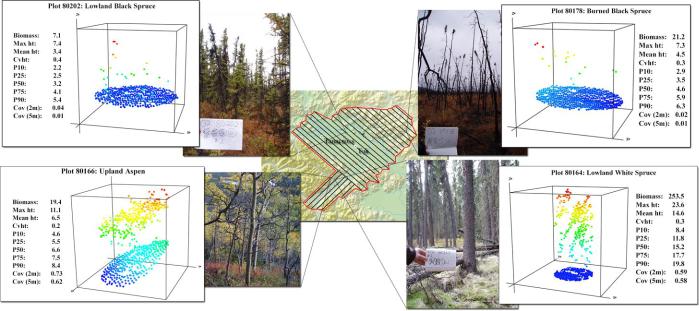
Given the structural and compositional complexity of many forests, there is a need for alternative techniques for quantifying biomass and aboveground carbon using LIDAR that are not dependent upon accurate detection and measurement of individual tree crowns. Aggregate measures of forest structure, including basal area (m2/ha), biomass (MG/ha), and volume (m3/ha), calculated from all trees within a given area (above a certain minimum diameter) are typically highly correlated to structural metrics calculated using the LIDAR point cloud data extracted over the same area. Most of the variability in biomass within a given area can be explained by three LIDAR-derived structural metrics: (1) mean height of canopy-level LIDAR returns, (2) LIDAR-derived percent canopy cover, and (3) standard deviation of canopy-level LIDAR returns [26]. Collectively, these three metrics provide a quantitative description of the three-dimensional spatial distribution of canopy material within a given area, which in turn, is strongly related to the amount of aboveground biomass present in this area. However, many other LIDAR-derived structural metrics can be generated from the LIDAR point cloud (maximum height of canopy level returns, 10th, 25th, 50th, 75th, 90th, percentile height of canopy-level returns, canopy density by layer, etc.). For example, Fig. 10.8 shows the vertical distribution of LIDAR data, extracted LIDAR structural metrics, and the biomass level for four selected field plots in interior Alaska. Magnussen and Boudewyn established the theoretical basis for the relationship between LIDAR height quantiles and the vertical distribution of canopy materials [29]. Given the tremendous variability in forest composition and structure in forests throughout the world, the specific models describing the relationship between biomass and LIDAR metrics can also vary by forest type, and often will incorporate different predictor variables and regression coefficients. A practical approach to estimate biomass and other inventory parameters (density, volume, etc.) using LIDAR was developed in Norway [35, 36], in which field inventory data was collected at a limited number of accurately-georeferenced plots, then empirical relationships were established between field-based inventory estimates and a selection of LIDAR structural metrics extracted for the area associated with each plot. An automated variable selection procedure (stepwise regression) was used to select the predictor variables for each regression model. Figure 10.9 shows the relationship between fieldand LIDARbased estimates of (square root-transformed) aboveground tree biomass on seventynine (79) field plots established in the upper Tanana valley of interior Alaska, where the model is obtained via a stepwise regression procedure.

Fig. 10.9 Relationship between (transformed) fieldand LIDAR-based estimates of aboveground tree biomass (MG/ha) for seventy-nine (79) plots in the upper Tanana valley of interior Alaska

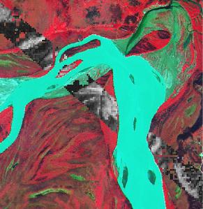
Fig. 10.10 Example of LIDAR-derived biomass measurements (black: low biomass, white: high biomass) within single LIDAR swath, upper Tanana valley of interior Alaska. Background is a false-color SPOT 5 image (2.5 meter resolution), and circles represent field plots (with same color ramp as the LIDAR grid cells)

This model is then applied to each grid cell within the LIDAR coverage area (where the grid cell size is a comparable grain size as the field plots (i.e. 1/30th hectare 18 m × 18 m grid cells) (see Fig. 10.10).

The LIDAR-based estimates of precision acquired over the coverage area can then be used to develop estimates of total (or mean) biomass. Due to the interest (to date) in using LIDAR to acquire better topographical information, most LIDAR