- •Table of Contents
- •About the Author
- •Dedication
- •Foreword
- •Acknowledgments
- •Why Does Office 365 Have Better Features?
- •Which Version of Office 365 Has Power Pivot?
- •Why Do I Have to Sign in to Excel?
- •How Can I Use Excel on Dual Monitors?
- •How Can I Open The Same Workbook Twice?
- •Find Icons on the Ribbon
- •Where is File, Exit?
- •Where Are My Macros?
- •Customizing the Ribbon
- •Go Wide
- •Minimize the Ribbon to Free Up a Few More Rows
- •Use a Wheel Mouse to Scroll Through The Ribbon Tabs
- •Why Do The Charting Ribbon Tabs Keep Disappearing?
- •Use Dialog Launchers For More Choices
- •Icon, Dropdowns, and Hybrids
- •Zoom is at the Bottom
- •Make Your Most-Used Icons Always Visible
- •The Excel 2003 Alt Keystrokes Still Work (If You Type Them Slowly Enough)
- •Use Keyboard Shortcuts to Access the Ribbon
- •Why Do I Have Only 65,536 Rows?
- •Which File Format Should I Use?
- •Why Does The File Menu Cover The Entire Screen?
- •How Do I Close The File Menu?
- •Increase the Number of Workbooks in the Recent Files List
- •Change All Print Settings in Excel
- •I Just Want The Old Print Preview Back
- •Get Quick Access to Formatting Options Using the Mini Toolbar
- •What Is Protected Mode?
- •Use a Trusted Location to Prevent Excel’s Constant Warnings
- •My Manager Wants Me to Create a New Expense Report from Scratch
- •Open a Copy of a Workbook
- •Open Excel with Ctrl+Alt+X
- •Have Excel Always Open Certain Workbook(s)
- •Set up Excel Icons to Open a Specific File on Startup
- •Use a Macro to Customize Startup
- •Control Settings for Every New Workbook and Worksheet
- •Excel Says I Have Links, But I Can Not Find Them
- •Automatically Move the Cell Pointer After Enter
- •Return to the First Column After Typing the Last Column
- •Enter Data in a Circle (Or Any Pattern)
- •How to See Headings as You Scroll Around a Report
- •How to See Headings and Row Labels as You Scroll Around a Report
- •Why is the Scrollbar Slider Suddenly Tiny?
- •Why Won’t My Scrollbar Scroll to My Charts?
- •Jump to the Edge of the Data
- •Jump to Next Corner of Selection
- •Ctrl+Backspace brings the Active Cell into View
- •Zoom with the Wheel Mouse
- •Copy a Formula to All Data Rows
- •A Faster Way To Paste Values
- •Quickly Turn a Range on Its Side
- •Quickly Rearrange Rows Or Columns
- •Quickly Copy Worksheets
- •Use Group Mode to Change All Worksheets
- •Find Text Numbers
- •Why Can’t Excel Find a Number?
- •Mix Formatting In A Single Cell
- •Enter a Series of Months, Days, or More by Using the Fill Handle
- •Have the Fill Handle Fill Your List of Part Numbers
- •Teach Excel to Fill A, B, C
- •Add Total to the End of Jan, Feb, ... Dec
- •Put Date & Time in a Cell
- •Use Excel as a Word Processor
- •Add Excel to Word
- •Use Hyperlinks to Create an Opening Menu for a Workbook
- •Spell check a Region
- •Stop Excel from AutoCorrecting Certain Words
- •Use AutoCorrect to Enable a Shortcut
- •Why Won’t the Track Changes Feature Work in Excel?
- •Simultaneously Collaborate on a Workbook with Excel Web App
- •How to Print Titles at the Top of Each Page
- •Print a Letter at the Top of Page 1 and Repeat Headings at the Top of Each Subsequent Page
- •How to Print Page Numbers at the Bottom of Each Page
- •How to Make a Wide Report Fit to One Page Wide by Many Pages Tall
- •Add a Printable Watermark
- •Print Multiple Ranges
- •Add a Page Break at Each Change in Customer
- •Save My Worksheet as a PDF File
- •Send an Excel File as an Attachment
- •Save Excel Data as a Text File
- •Close All Open Workbooks
- •I Just Closed an Unsaved Workbook
- •Roll Back to an AutoSaved Version
- •Have Excel Talk to You
- •Enter Special Symbols
- •What Do All the Triangles Mean?
- •Why does Excel Insert Cell Addresses When I Edit In a RefEdit Box?
- •F4 Repeats Last Command
- •Print all Excel Keyboard Shortcuts
- •Create a Personal Macro Workbook
- •Macro to Toggle Positive to Negative
- •Assign a Macro to a Shortcut Key
- •Assign a Macro to a Toolbar Icon
- •Use a Macro to Change Case to Upper, Lower, or Proper
- •Get Free Excel Help
- •Start a Formula with = or +
- •Three Methods of Entering Formulas
- •Why Does Excel 2013 Look Like A Slot Machine?
- •Use Parentheses to Control the Order of Calculations
- •Long Formulas in the Formula Bar
- •Copy a Formula That Contains Relative References
- •Copy a Formula While Keeping One Reference Fixed
- •Create a Multiplication Table
- •Calculate a Sales Commission
- •Simplify the Entry of Dollar Signs in Formulas
- •Learn R1C1 Referencing to Understand Formula Copying
- •Create Easier-to-Understand Formulas with Named Ranges
- •See All Named Ranges at 39% Zoom
- •Use Named Constants to Store Numbers
- •Total Without Using a Formula
- •Add or Multiply Two Columns Without Using Formulas
- •Type 123 to Enter 1.23
- •Join Two Text Columns
- •Concatenate Several Cells
- •Join Text with a Date or Currency
- •Break Data Apart Using Flash Fill
- •Parse Data using Text to Columns
- •Excel Is Randomly Parsing Pasted Data
- •I Lose Leading Zeroes From CSV Files
- •Open CSV File With Dates in D/M/Y Format
- •Handle Dates in YYYYMMDD format
- •My G/L Software Uses a Trailing Minus for Negative Numbers
- •Parse Data With Leader Lines
- •Parse Multi-Line Cells
- •Change Smith, Jane to Jane Smith
- •Convert Numbers to Text
- •Fill a Cell with Repeating Characters
- •CLEAN Hasn’t Kept Up With The Times
- •Add the Worksheet Name as a Title
- •Use AutoSum to Quickly Enter a Total Formula
- •AutoSum Doesn’t Always Predict My Data Correctly
- •Use the AutoSum Button to Enter Averages, Min, Max, and Count
- •Ditto The Formula Above
- •The Count Option of the AutoSum Dropdown Doesn’t Appear to Work
- •Total the Red Cells
- •Automatically Number a List of Employees
- •Automatically Number the Visible Rows
- •Discover New Functions Using the fx Button
- •Get Help on Any Function While Entering a Formula
- •Use F9 in the Formula Bar to Test a Formula
- •Quick Calculator
- •When Entering a Formula, You Get the Formula Instead of the Result
- •Highlight All Formula Cells Using Conditional Formatting
- •You Change a Cell in Excel but the Formulas Do Not Calculate
- •Calculate One Range
- •Why Use the Intersection Operator?
- •Understand Implicit Intersection
- •Find the Longest Win Streak
- •Add B5 On All Worksheets
- •Consider Formula Speed
- •Exact Formula Copy
- •Calculate a Loan Payment
- •Calculate Many Scenarios for Loan Payments
- •Back into an Answer Using Goal Seek
- •Create an Amortization Table
- •Do 40 What-if Analyses Quickly
- •Random Walk Down Wall Street
- •What-If For 3 Or More Variables
- •Rank Scores
- •Round Numbers
- •Round to the Nearest $0.05 with MROUND
- •Round Prices to the Next Highest $5
- •Round 0.5 towards Even Per ASTM-E29
- •Separate the Integer From the Decimals
- •Why Is This Price Showing $27.85000001 Cents?
- •Calculate a Percentage of Total
- •Calculate a Running Percentage of Total
- •Use the ^ Sign for Exponents
- •Raise a Number to a Fraction to Find the Square or Third Root
- •Calculate a Growth Rate
- •Find the Area of a Circle
- •Figure Out Lottery Probability
- •Help Your Kids with Their Math
- •Convert Units
- •XOR Only Works Correctly for Two Values
- •Find the Second Largest Value
- •Format Every Other Row in Green
- •\Use IF to Calculate a Bonus
- •IF with Two Conditions
- •Tiered Commission Plan with IF
- •Display Up/Down Arrows
- •Stop Showing Zeroes in Cell Links
- •Count Records That Match a Criterion
- •Build a Table That Will Count by Criteria
- •Sum Records That Match a Criterion
- •Can the Results of a Formula Be Used in SUMIF?
- •Calculate Based on Multiple Conditions
- •Avoid Errors Using IFERROR
- •Use VLOOKUP to Join Two Tables
- •Every VLOOKUP Ends in False
- •Lookup Table Does Not Have to Be Sorted
- •Beware of #N/A from VLOOKUP
- •Add New Items to the Middle Of Your Lookup Table
- •Consider Naming the Lookup Table
- •Remove Leading and Trailing Spaces
- •Your Lookup Table Can Go Across
- •Copy a VLOOKUP Across Many Columns
- •INDEX Sounds Like an Inane Function
- •You Already Know MATCH, Really!
- •INDEX Sounds Like an Inane Function - II
- •VLOOKUP Left
- •Fast Multi-Column VLOOKUP
- •Speed Up Your VLOOKUP
- •Return the Next Larger Value in a Lookup
- •Two-Way Lookup
- •Combine Formulas into a Mega-Formula
- •Combine Two Lists Using VLOOKUP
- •Watch for Duplicates When Using VLOOKUP
- •Return the Last Entry
- •Return the Last Matching Value
- •Sum All of the Lookups
- •Embed a Small Lookup Table In Formula
- •I Don’t Want to Use a Lookup Table to Choose One of Five Choices
- •Is there Something More Flexible than CHOOSE?
- •Lookup Two Values
- •Add Comments to a Formula
- •Create Random Numbers
- •Randomly Sequence a List
- •Play Dice Games with Excel
- •Generate Random Without Repeats
- •Calculate a Trendline Forecast
- •Forecast Data with Seasonality
- •Build a Model to Predict Sales Based on Multiple Regression
- •Switching Columns into Rows Using a Formula
- •SUM a Range that is C5 Rows Tall Using OFFSET
- •Replace Volatile OFFSET with INDEX
- •How Can You Test for Volatility?
- •Whatever Happened to the @@ Function?
- •Tables Are Like a Database in Excel
- •Dealing with Table Formulas
- •Rename Your Tables
- •Charts , VLOOKUP & Pivots Expand With The Table
- •Before Deleting a Cell, Find out if Other Cells Rely on It
- •Calculate a Formula in Slow Motion
- •Which Cells Flow into This Cell?
- •Color all Precedents or Dependents
- •Monitor Distant Cells
- •Auditing Worksheets with Inquire
- •Use Real Dates
- •How Can I Tell If Have Real Dates?
- •Convert Text Dates to Real Dates
- •Format Dates
- •Format Dates As Quarters or Weeks
- •Display Monthly Dates
- •Add a Column to Show Month or Weekday
- •Calculate First of Month
- •Calculate the Last Day of the Month
- •Calculate Invoice Due Dates
- •Calculate Receivable Aging
- •NOW, or TODAY?
- •Find the Last Sunday Of the Month
- •Calculate Work Days
- •Calculate Work Days for a Farmers Market
- •Calculate Age in Years, Months, Days
- •Coerce an Array of Dates from 2 Dates
- •Use Real Times
- •Strangeness of Time Formatting
- •Convert Time to Decimal Hours
- •Calculate with Time
- •Enter Minutes and Seconds
- •Convert Text to Time
- •Can Excel Track Negative Time?
- •Fill Blanks With Value Above
- •See Formulas in Excel 2013
- •Create a Bell Curve in Excel
- •Change from Lower to Upper Case in Excel
- •Spell Out Numbers in Excel
- •Copy Macro Code from the Internet Into an Add-In
- •Return Data from a Webservice in Excel 2013
- •Add New Functions to Excel with Fast Excel SpeedTools Extras
- •=SUM(B1:B5) is Better Than =B1+B2+B3+B4+B5
- •How to Set up Your Data for Easy Sorting and Subtotals
- •How to Fit a Multiline Heading into One Cell
- •No Tiny Blank Columns Between Columns
- •How to Sort Data
- •Sort Days of the Week
- •Sort a Report into a Custom Sequence
- •Sort All Red Cells to the Top of a Report
- •Sort Pictures With Data
- •Quickly Filter a List to Certain Records
- •Use Search While Filtering
- •Filter by Selection
- •Use AutoSum After Filtering
- •Filter Only Some Columns
- •Find the Unique Values in a Column
- •Use Advanced Filter
- •Replace Multiple Filter Criteria with a Single Row of Formulas
- •Add Subtotals to a Data set
- •Use Group & Outline Buttons to Collapse Subtotaled Data
- •Manually Apply Groups
- •Group Report Sections
- •Copy Just Totals from Subtotaled Data
- •Sort Largest Customers to the Top
- •Select 100 Columns in Subtotals
- •Enter a Grand Total of Data Manually Subtotaled
- •Add Other Text to the Subtotal Lines
- •Subtotals by Product Within Region
- •Format the Subtotal Rows
- •My Manager Wants a Blank Line After Each Subtotal
- •Subtotal One Column and Count Another Column
- •Can You Get Medians?
- •Horizontal Subtotals
- •Be Wary
- •Send Error Reports
- •Help Make Excel Better
- •Remove Blank Rows from a Range
- •Remove Blanks from a Range While Keeping the Original Sequence
- •Double Space Your Data Set
- •Use Find to Find an Asterisk
- •Use an Ampersand in a Header
- •Hide Zeros & Other Custom Number Formatting Tricks
- •Use Consolidation to Combine Two Lists
- •Combine Four Quarterly Reports
- •Find Total Sales by Customer by Combining Duplicates
- •Remove Duplicates
- •Preview Remove Duplicates Without Removing Them
- •Protect Cells That Contain Formulas
- •Find Differences In Two Lists
- •Number Each Record, Starting at 1 for a New Customer
- •Deal with Data in Which Each Record Takes Five Physical Rows
- •Add a Customer Number to Each Detail Record
- •Use a Built-in Data Entry Form
- •Cell AutoComplete Stopped Working
- •Data Cleansing with Flash Fill in Excel 2013
- •Flash Fill was there and is now Gone
- •Flash Fill Was Not Perfect
- •Flash Fill Won’t Fill Numbers
- •Flash Fill and Dates
- •Flash Fill and Ambiguous Data
- •Use a Pivot Table to Summarize Detailed Data
- •Your Manager Wants Your Report Changed
- •Add or Remove Fields from an Existing Pivot Table
- •Summarize Pivot Table Data by Three Measures
- •Why Does the Pivot Table Field List Keep Disappearing?
- •Move or Change Part of a Pivot Table
- •See Detail Behind One Number in a Pivot Table
- •Use Multiple Value Fields as a Column or Row Field
- •Update Data Behind a Pivot Table
- •Why do I Get a Count Instead of a Sum?
- •Convert Your Data to a Table Before Adding Records
- •Create a Flattened Pivot Table for Reuse
- •Replace Blanks in a Pivot Table with Zeros
- •Collapse and Expand Pivot Fields
- •Specify a Number Format for a Pivot Table Field
- •Preserve Column Widths
- •Show Yes/No in a Pivot Table
- •Pivot Table Format Defaults
- •Format Pivot Tables with the Gallery
- •None of the 46,273 Built-In Styles Do What My Manager Asks For
- •Select Pivot Table Parts For Formatting
- •Apply Conditional Formatting to a Pivot Table
- •Can I Save Formatting in a Template?
- •Manually Re-sequence the Order of Data in a Pivot Table
- •Present a Pivot Table in High-to-Low Order by Revenue
- •Excel 2016 Sometimes Auto-Groups Daily Dates to Month
- •Group Daily Dates by Month in a Pivot Table
- •Create a Year-Over-Year Report
- •Group by Week in a Pivot Table
- •Limit a Pivot Report to Show Just the Top 5 Customers
- •Build a Better Top Five Using Groups
- •Build a Better Top Five with A Filter Hack
- •Build a Better Top 5 Using the Data Model
- •Limit a Report to Just One Region
- •Create an Ad-Hoc Reporting Tool
- •Create a Report for Every Customer
- •Create Pivot Charts
- •Add Visual Filters to a Pivot Table or Regular Table
- •Run Many Pivot Tables From one Slicer
- •Filter Dates Using a Timeline in Excel 2013 & Newer
- •Group Employees Into Age Bands
- •Create a Frequency Distribution
- •Grouping 1 Pivot Table Groups Them All
- •Reduce Size 50% Before Sending
- •Drag Fields to the Pivot Table
- •Create a Report That Shows Count, Min, Max, Average, Etc.
- •Better Calculations with Show Values As
- •Pivot Ranks Don’t Match RANK()
- •Calculated Fields in a Pivot Table
- •Add a Calculated Item to Group Items in a Pivot Table
- •Group Text Fields to Build Territories
- •Calculations Outside of Pivot Tables
- •Show Customer Account & Name
- •Show Months with Zero Sales
- •Create a Unique List of Customers with a Pivot Table
- •Use a Pivot Table to Compare Two Lists
- •Use a Pivot Table When There Is No Numeric Data
- •Fix Misspelled Customer Names
- •Create a Pivot Table from Access Data
- •What Happened to Multiple Consolidation Ranges in Pivot Tables?
- •What are the Products in Power BI And How Can I Get Them?
- •Know if You Have 32-Bit or 64-Bit Excel
- •Load and Clean Data with Power Query
- •Power Query is Easier to Learn than VBA Macros
- •I Have More than 1,048,576 Rows of Data
- •Load a List of File Names into Excel
- •Load a Folder of CSV Files into a Single Excel Worksheet
- •My Headings Repeat Every 60 Rows
- •Fill in Blanks with Values from Above
- •Use Power Query to Clean Data Already in Excel
- •Pivot from Multiple Tables in Excel 2013 Data Model
- •Reporting from the Smaller Side of the Relationship
- •Use Joiner Tables Between Tables
- •Five Reasons to Use Power Pivot
- •Why Isn’t Power Pivot Tab in the Ribbon?
- •Get Excel Data Into Power Pivot
- •Open the Power Pivot Window
- •Define Relationships Between Tables
- •Sort Month Name by Month Number
- •Create a Calendar Table
- •The Formulas are called DAX
- •Adding Calculations In the Power Pivot Grid
- •Refer to a Related Table in a Formula
- •Creating the Power Pivot Table
- •Building the Pivot Table
- •Feature X Won’t Work in Power Pivot
- •Replace Calculated Fields with DAX
- •Calculate() is Like SUMIFS()
- •Unapply a Filter Using DAX
- •Unfilter Using Time Intelligence
- •Convert Power Pivot to Formulas
- •January Actuals and February Plan
- •Power View Is Replaced with Power BI
- •Power BI Transforms Excel Data into Interactive Dashboards
- •First POwer BI Step: Get a Free Account for Power BI
- •Optional Step 1: Take the Sample Dashboards for a Spin
- •Use Q&A to Investigate Your Data
- •Click a Dashboard Element to Open the Underlying Report
- •Click in one Chart to Filter Other Charts
- •Enable Drill-Down Mode
- •Sorting is Hidden Behind More Options
- •Optional Step 2: Connect to an Existing Service
- •Download Power BI Desktop to Your Computer
- •Prepare Your Excel Data for Power BI
- •Add a Calendar Table
- •Three Icons in Power BI Desktop
- •In Power BI Desktop, the Power Query Tools Are Called Get Data
- •Load Your Excel Data to Power BI Desktop
- •In Power BI Desktop, the Power Pivot tools are called Modeling
- •Define Relationships in Power BI Desktop
- •Classify Your Geography Fields in Power BI Desktop
- •Prevent Power BI from Adding Up Year Fields
- •Sort This by That
- •Define Synonyms in Power BI Desktop
- •Hide Columns So They Can't Be Chosen
- •Three Ways to BUild Visualizations in a Report
- •FOrmatting a Chart
- •Add Lines using Analytics
- •Adding More Visualizations to a Page
- •It is Insanely Easy to Build a Hierarchy
- •Open Source Visualizations
- •Every Chart is a Slicer For Other Charts
- •A Report Can Have Multiple Pages
- •Using Maps in Power BI Desktop
- •Three Types of Filters
- •Where is the Top 10 Filter?
- •Add Titles, Logos, & Embelishments
- •Don't Forget to Save Your File!
- •Share Your Dashboard to Power BI in the Cloud
- •Use Quick Insights
- •View Your Report in a Browser
- •Q&A Works on Dashboards, Not Reports
- •Share a Dashboard With Your Manager
- •Wait a Second - a Sharing Link? Isn't this Dangerous?
- •Consume Your Dashboard Using Power BI Mobile
- •What Does All Of This Cost?
- •How Do I Update My Dashboard Every Day?
- •That's All For Power BI In This Book
- •Put a Pivot Table on a Map In Excel 2013 Power Map
- •Tricks for Navigating the Map in Power Map
- •Fine-Tuning Power Map
- •Creating a Video from Power Map
- •Use an Alternate Map for Power Map
- •Filtering in Power Map
- •Excel Data to Mailing Labels in Word
- •Excel 2013 Allows Slicers on Regular Tables
- •Use Power Query to Load Many Web Pages
- •Create a Chart with One Click
- •Teach Excel Your Favorite Chart
- •Move a Chart
- •Copy a Chart Detached from the Data
- •Add New Data to a Chart
- •Excel 2013 Offers Easy Chart Formatting
- •Begin Excel 2010 Formatting on Design
- •The Chart Layout Tab Is Missing in Excel 2013
- •Formatting Charts in Excel 2010 with Layout
- •Legend At the Top
- •The 2010 Format Dialog Box is a Task Pane in 2013
- •Display an Axis in Millions
- •Select Anything on a Chart to Format
- •The Format Dialog Box Offers a New Trick
- •Use Meaningful Chart Titles
- •Avoid 3-D Chart Types
- •Prevent the Drop to Zero
- •Explode One Slice of the Pie
- •Move Small Pie Slices To Second Chart
- •Add a Trendline to a Chart
- •See Detail on Large & Small Data Points
- •Chart Two Series with Differing Orders of Magnitude
- •Hide Subtotals From Chart in Excel 2013
- •Create Pivot Charts from Detail Data in Excel 2013
- •Use Formulas for Chart Labels in Excel 2013
- •Interactive Chart to Show One Customer
- •Tie the Chart Title to a Cell
- •Excel 2016 Adds a Waterfall Chart
- •Use an Invisible Series to Float Columns
- •Use Rogue Series for Shading
- •Two Stacked, One Clustered Column
- •Conditional Format a Chart
- •Scatter Charts are Versatile But Require a Different Workflow
- •When do I Use Which Chart Type?
- •Track Sales Leads with a Funnel Chart
- •Create Tiny Charts with Sparklines
- •Sparklines Are Not Scaled Together
- •What is the Win Loss Sparkline For?
- •Labeling Sparklines
- •Shade the Normal Range in a Sparkline
- •Convert a Table of Numbers to a Visualization
- •Control Values for Each Icon
- •Add Icons to Only the Good Cells
- •Use the SIGN Function for Up/Flat/Down Icon Set
- •Data Bars Options
- •Comparative Histogram
- •Select Every Kid in Lake Wobegon
- •There is a Font Optimized for Excel
- •Show Checkmarks in Excel
- •Add Bullets to Excel
- •Use the Border Tab in Format Cells
- •Remove Borders from Filled Cells
- •Double Underline a Grand Total
- •Why Did the Colors Change in Excel 2013?
- •Where Are My Excel 2003 Colors?
- •Transform Black-and-White Spreadsheets to Color by Using a Table
- •Fit a Slightly Too-Large Value in a Cell
- •Turn Off Wrap Text in Pasted Data
- •Delete All Pictures in Pasted Data
- •Prevent Long Text from Spilling
- •Show Two Values in a Split Cell
- •For Each Cell in Column A, Have Three Rows in Column B
- •Show Results as Fractions
- •Better Scientific Notation
- •Fill a Cell with Asterisks
- •I type 152 and get 1.52
- •Use Cell Styles to Change Formats
- •Move Columns by Sorting Left to Right
- •Move Columns Using Insert Cut Cells
- •Move Rows or Columns with Shift Drag
- •Select All Cells Using the Keyboard
- •Change the Width of All Columns with One Command
- •Copy Column Widths to a New Range
- •Copy Row Heights
- •Use White Text to Hide Data
- •Hide Values Using a Number Format
- •Hide and Unhide Data
- •Group Columns Instead of Hiding Them
- •Hide Error Cells When Printing
- •Unhide All Sheets
- •Very Hide a Worksheet
- •Organize Your Worksheet Tabs with Color
- •Copy Formatting to a New Range
- •Copy Without Changing Borders
- •Power Up Format Painter
- •Fill Formatting
- •Change All Red Font Cells to Blue Font
- •Replace Partially Bold Cells
- •Change the Look of Your Workbook with Document Themes
- •Create Your Own Theme
- •Bring Back the Office 2010 Colors And Shiny Objects
- •Change the Background of a Worksheet
- •Add a Printable Background to a Worksheet
- •Remove Hyperlinks Automatically Inserted by Excel
- •Select a Hyperlink Cell Without Following the Hyperlink
- •Pasted URLs Don’t Become Hyperlinks
- •Debug Using a Printed Spreadsheet
- •Change the Appearance of Cell Comments
- •Control How Your Name Appears in Comments
- •Force Some Comments to ALWAYS Be Visible to Provide a Help System
- •Change the Comment Shape to a Star
- •Add a Pop-up Picture of an Item in a Cell
- •Add a Pop-up Picture to Multiple Cells
- •Build Reports Where Columns in Each Section 1 Don’t Line Up
- •Paste a Live Picture of a Cell
- •Add Formatting to Pictures in Excel
- •Remove Picture Background
- •Inserting a Screen Clipping
- •Draw an Arrow to Visually Illustrate That Two Cells Are Connected
- •Add Connectors to Join Shapes
- •Circle a Cell on Your Worksheet
- •Draw Perfect Circles
- •Add Text to Any Closed Shape
- •Place Cell Contents in a Shape
- •Rotate a Shape
- •Create Dozens of Lightning Bolts
- •Make a Logo into a Shape
- •Draw Business Diagrams with Excel
- •Choose the Right Type of SmartArt
- •Use the Text Pane to Build SmartArt
- •Change a SmartArt Layout
- •Format SmartArt
- •Switch to the Format Tab to Format Individual Shapes
- •Use Cell Values as the Source for SmartArt Content
- •Add WordArt to a Worksheet
- •Chart and SmartArt Text Is Automatically WordArt
- •Excel 2013 Offers an Excel App Store
- •Add a Dropdown to a Cell
- •Configure Validation to “Ease up”
- •Use Validation to Prevent Duplicate Data Entry
- •Use Validation to Create Dependent Lists
- •Add a ToolTip to a Cell to Guide the Person Using the Workbook
- •Combine Validation with AutoComplete
- •Afterword
- •Index
32 |
POWER EXCEL WITH MR EXCEL |
|
|
Figure 69 Double-click the bottom of the active cell.
Result: Excel will navigate down until the cell before a blank cell.
Additional Details: Double-click the right edge of the active cell to move to the right edge of the data.
Alternate Strategy: For keyboard fans, using Ctrl+Down Arrow or pressing End followed by the Down Arrow will do the same thing.
JUMP TO NEXT CORNER OF SELECTION
Problem: I have a large column of numbers stored as text. I like to use the error correction dropdown that appears next to the first cell in the selection in order to convert the text to numbers. However, if I choose the first cell, then select the range with Ctrl+Shift+Down Arrow, I can no longer see the error dropdown.
Figure 70 If you select more than a screen of data, you can not see this icon at the top of the range.
Strategy: Pressing Ctrl+Period will keep your selection, but move the active cell to the next corner of the selection. This is a great way to see the top of your selection, including the error icon.
If you have a single-column range selected, a single Ctrl+Period will get you to the top. If you have a rectangular range selected, pressing Ctrl+Period will move in a clockwise sequence to the next corner.
If the active cell is currently in the bottom-right, it might require you to press Ctrl+Period twice.
Additional Details: If you press Ctrl+Period to return to the top, then press it again to return to the bottom, the error icon remains in view. This suggests that the intention was to show the error icon even in the original case, but a bug is preventing it.
Figure 71 The active cell moves clockwise to the next corner.
CTRL+BACKSPACE BRINGS THE ACTIVE CELL INTO VIEW
Problem: I keep selecting my data set using Ctrl+Shift+DownArrow. Now I can’t see the active cell.
Strategy: Ctrl+Backspace will scroll the active cell back into view.
PART 1: THE EXCEL ENVIRONMENT |
|
33 |
|
|
|
|
ZOOM WITH THE WHEEL MOUSE |
Problem: I have to constantly zoom in and out on my worksheet. The zoom slider is a hassle.
Strategy: Hold down the Ctrl key while rolling the mouse wheel. Roll away from you to zoom in. Roll towards you to zoom out.
Additional Details: Most people use the scroll wheel to scroll up and down. Did you know that you can also use the mouse to scroll side to side? Click and hold the mouse wheel then move the mouse left or right to scroll sideways. This only works when you have a horizontal scrollbar available.
COPY A FORMULA TO ALL DATA ROWS
Problem: I have a worksheet with thousands of rows of data. I often enter a formula in a new column and need to copy it down to all of the rows. I try to do this by dragging the fill handle. But as I try to drag, Excel starts accelerating faster and faster. Before I know it, I’ve overshot the last row by thousands of rows. I
start dragging back up. Again, Excel starts accelerating. Soon, the cell pointer is moving somewhere close 1 to the speed of sound, and I find that I’ve overshoot the last row in the other direction. I end up going down
and up, down and up. I call this frustrating process the “fill handle dance.” Is there a way to stop the mad- ness?
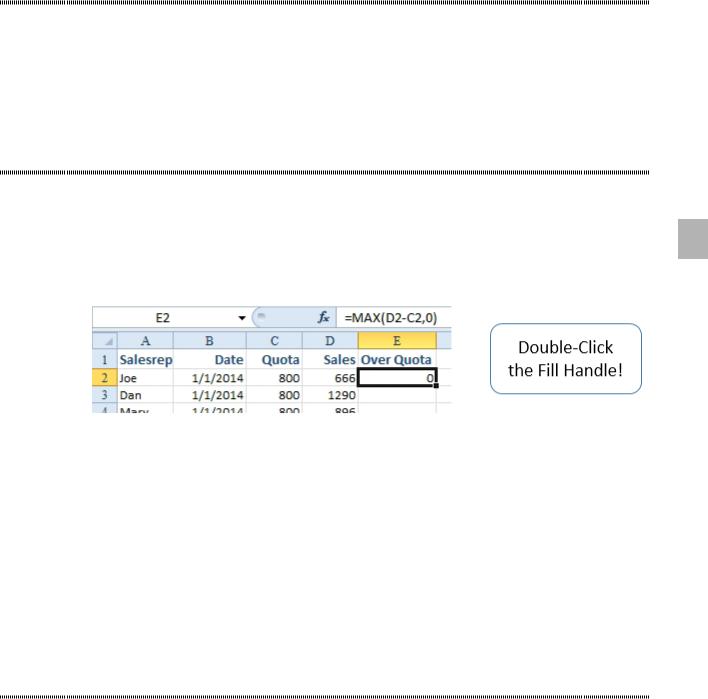
Figure 72 Copy this formula all the way down.
Strategy: You can very quickly copy a formula down to all the rows by double-clicking the fill handle. Excel will copy the formula down until it encounters a blank row in the adjacent data. The fill handle is the square dot in the lower-right corner of the cell pointer box. When you hover your mouse over the fill handle, the cell pointer changes to a plus.
Gotcha: In Excel 2007 and earlier, a single blank cell in the adjacent column would cause the copy action to stop prematurely. If the adjacent column is particularly sparse, you could hide that column and then Excel would look at the next visible column to the left. This algorithm was improved in Excel 2010 and will usually get you to the bottom of the data.
Alternate Strategy: From E2, press Left Arrow to go to D2. Ctrl+Down Arrow to get to the bottom, Press
Right Arrow to go back to column E. Ctrl+Shift+Up Arrow selects from the last row to E2. Ctrl+D will fill down and the formula in E2 will get copied. Practice for a week, and you can do all the keystrokes in less than a second. You will be on the team if Excel ever becomes an Olympic sport.
COPY THE CHARACTERS FROM A CELL INSTEAD OF COPYING AN ENTIRE CELL
Problem: I need to copy from Excel to Outlook. Microsoft applies weird formatting to the values when I paste to Outlook. Instead of getting just the text, it almost seems like Outlook is wrapping the cell value in a table. I end up pasting Excel data to Notepad, then copying from Notepad.
Strategy: If you have a single cell to copy and want to grab just the characters from the cell, you follow these steps:
1. Select the cell. Put the cell in Edit mode by pressing F2. 2. Select all the characters in the cell by pressing Ctrl+A.
3. Press Ctrl+C to copy.
4. Paste to another application. Excel will not try to place the text in a table.
An advantage of this method is that characters copied to the Clipboard will remain on the Clipboard longer than cells copied to the Clipboard. If you copy a cell, the Clipboard is cleared when you press Esc or save the file. If you copy characters to the Clipboard, they will stay on the Clipboard after these events.
34 |
POWER EXCEL WITH MR EXCEL |
|
|
Alternate Strategy: If you have several cells to copy, you can just copy and paste the cells. After you paste to Outlook, a Paste Options icon will appear. You can open the icon and choose Keep Text Only to convert the table to text.
After converting the pasted cells to text, you will have plain text that appears as if you simply typed the values
A FASTER WAY TO PASTE VALUES
Problem: I have a range of formulas that I need to convert to values.
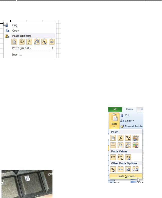
Strategy: Use the Paste Values icon on the right-click menu. You will see that the right-click menu in- cludes icons for Paste, Paste Values, Paste Formulas, Transpose, Paste Formats, and Create Links.
Figure 73 The right-click menu offers 6 options.
When you hover over one of those icons, the rest of the context menu disappears so that you can see the effect of the paste in Live Preview. If you hover over Paste Special in the right-click menu, the menu will disappear and you have access to all 15 icons.
If you prefer to use the mouse, try this amazing trick: hold down the shift key while you drag the border of a selection. When you release the mouse, choose Copy Here as Values Only from the menu that appears.
If you regularly use the Paste icon in the Home tab, the dropdown at the bottom of the tab now leads to a menu with the 15 icons. There are still some options in Paste Special that are not available in the icons. You can access those commands by using the Paste Special menu item at the bottom of this figure.
Many times each day, I convert formulas to values by using Ctrl+C,
Alt+E+S+V, Enter.
Sometimes, I need to copy values and formats to a new place. In the new place, I have to do Alt+E+S+V, Enter, Alt+E+S+T+Enter.
As mentioned previously, you can use Ctrl+C, Ctrl+V, Ctrl, V to change formulas to value. To paste values and formats, you now use the new Ctrl+V, Ctrl, E to paste values and number formatting.
PeopleinmyseminarstellmetouseAlt,H,V,VortouseCtrl+Alt+V,
V.
There might be an even faster way. This key is the right-click key.
Use Ctrl+C, Right-Click Key, V to paste as values. If you don’t have the Right-Click key, use Shift+F10. If you need to paste values and formats, the Right-Click, E keys will do it.
Figure 74 The paste dropdown offers the icons.
PART 1: THE EXCEL ENVIRONMENT |
|
35 |
|
|
|
|
|
||
The one complaint that I have heard about the Paste Op- |
|
|
||
tions menu is that it is tough to figure out what the icons |
|
|
||
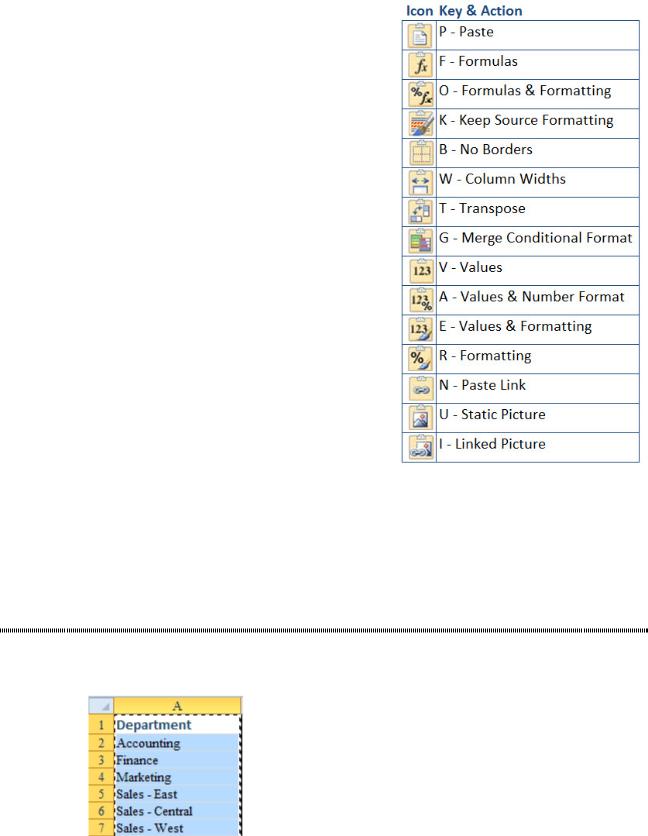
mean. Photocopy Figure 75 and hang it up by your desk. |
|
|
||
The following list describes each of the 15 items in the |
|
|
||
Paste Options menu: |
|
|
||
●● |
Paste is a regular paste. You get formulas, borders, |
|
|
|
●● |
and formats. |
|
|
|
Formulas pastes the formulas. It will not change |
|
|
||
●● |
formatting. |
|
|
|
Formulas & Formatting will paste the formulas |
|
|
||
|
and any numeric formatting. Borders, comments, |
|
|
|
●● |
and fills are not pasted. |
|
|
|
Keep Source Formatting is similar to a regular |
|
|
||
|
paste. |
|
|
|
●● |
No Borders pastes everything except for the bor- |
|
|
|
|
1 |
|||
|
ders. |
|
||
●● |
Column Widths copies the column widths from the |
|
|
|
|
|
|||
●● |
source range. |
|
|
|
Transpose turns data sideways. Rows become col- |
|
|
||
|
umns. |
|
|
|
●● Merge Conditional Formatting allows you to mix |
|
|
||
●● |
two different conditional formats. |
|
|
|
Values eliminates the formulas and paste their cur- |
|
|
||
●● |
rent values. |
|
|
|
Values & Number Format converts formulas to |
|
|
||
|
values, but brings along any numeric formatting ap- |
|
|
|
●● |
plied to the source range. |
|
|
|
Values & Formatting converts formulas to values, |
|
|
||
|
but brings along the cell formatting, too. |
|
|
|
|
Figure 75 Keys in Paste Options menu. |
|||
●● |
Formatting pastes only the formats. |
|
|
|
●● |
Paste Link will create formulas in the pasted range that point back to the source range. |
|
|
|
●● |
Static Picture pastes a picture of the copied range. This picture might include cells, SmartArt, |
|||
●● |
charts, and so on. When the original range changes, this picture does not change. |
|
|
|
Linked Picture pastes a live picture of the copied range. When something changes in the original |
||||
|
range, the picture reflects that change. This used to be called the Camera Tool in Excel 2003. |
|
|
QUICKLY TURN A RANGE ON ITS SIDE
Problem; I have a column that contains 20 department names going down a column. I need to build a worksheet with those names going across row 1.
Strategy: Copy the data. Select a new blank cell. Do a Paste
Transpose. Here’s how:
1. Highlight the department names in column A.
2. Ctrl+C to copy the cells to the Clipboard.
3. Move the cell pointer to a blank area of the worksheet.
Your paste region can not start in the same cell as your copy region.
4. Open the Paste dropdown. Click the Transpose icon.
Figure 76 Turn this data sideways.