

162 |
POWER EXCEL WITH MR EXCEL |
|
|
|
BEWARE OF #N/A FROM VLOOKUP |
Problem: A few of my VLOOKUPs are giving me the #N/A error.
Figure 402 BG33-9 is a new item and isn’t in the lookup table.
Strategy: This is common when you are doing VLOOKUP. It tells you that the lookup value is not found in the first column of the table. When you encounter an #N/A error, add that item to the table (see the next topic).
Additional Details: To isolate the #N/A errors, sort your data descending (using the ZA icon). All of the #N/A errors will sort to the top.
Additional Details: If you don’t want to update the lookup table with new values, but prefer to have alternate text entered, use IFERROR:
=IFERROR(VLOOKUP(),”Item Not Found”).
Gotcha: If you leave the #N/A errors in the data set and try to add up that column, the SUM will be #N/A. One single #N/A causes all downline formulas to calculate as #N/A.
ADD NEW ITEMS TO THE MIDDLE OF YOUR LOOKUP TABLE
Problem: I have to add BG33-9 to my lookup table. When I enter it in row 31, the #N/A error does not go away.
Strategy: You would have to rewrite the VLOOKUP to point to $L$3:$M$30. Instead, you could use any of these clever strategies:
●● Insert new cells anywhere in the middle of your lookup table. For example choose L7:M7 and do Alt+I+E followed by Enter. This will Insert Cells and shift the remaining items down.
●● Specify L:M as the lookup table. This uses the whole column as the lookup table. Now, you can add items to the bottom without rewriting the formula. Excel is smart enough to only use the non-blank cells when calculating.
●● Ctrl+T the lookup table before you add new values. When you type new values in row 31, the table expands to include the new row. In one of those scary bits of Excel magic, they actually rewrite your formulas to point to the extra row in the VLOOKUP formula. This happens even if you are not using
Table Formula Nomenclature.
CONSIDER NAMING THE LOOKUP TABLE
Problem: My lookup table is on another worksheet. The VLOOKUP is really confusing =VLOOKUP(A2,’Lookup Table Sheet’!$A$2:$B$30,2,FALSE).
Strategy: Many people in my live seminars say that they use a range name to name the lookup table.
Go to your Lookup Table Worksheet. Select cells A2:B30. Click in the Name Box to the left of the formula bar. Type a simple name like ProdTable and press Enter. Remember - the name can not contain a space. ProdTable or Prod_Table are OK. Prod Table is not.
Future VLOOKUPs can be entered as: =VLOOKUP(A2,ProdTable,2,FALSE). This is simpler to enter.
REMOVE LEADING AND TRAILING SPACES
Problem: None of my VLOOKUP formulas are working. I can clearly see that there is a match in the lookup table, but Excel cannot see it.
PART 2: CALCULATING WITH EXCEL |
163 |
|
|
Figure 403 None of the VLOOKUP functions work.
Strategy: A common problem is that either the item in column A or Column L has trailing spaces. This can happen if you downloaded the data from another system.
To fix this problem, you select cell A2 and press the F2 key to put the cell in Edit mode. A flashing insertion cursor will appear at the end of the cell. Check to see if the insertion cursor appears immediately after the last character or a few spaces away.
Edit cell L2 to see if there are trailing spaces. You will likely |
|
|
find that either column has trailing spaces. Below, you can |
|
|
see that there are a couple trailing spaces after the Item in |
|
|
column A. These trailing spaces cause the VLOOKUP to |
|
|
not classify the cells as a match. Although you can tell that |
|
2 |
“BG33-8 ” is the same as “BG33-9”, Excel cannot. |
Figure 404 Column A has trailing spaces. |
You can use the TRIM function to remove leading and trailing spaces from a value. If there are spaces between words, it will change consecutive spaces to a single space. For example, =TRIM(“ Bill Jelen ”) would change the cell contents to “Bill Jelen”.
Additional Details: If the trailing spaces appear in your lookup value, use TRIM around that one value.
Change =VLOOKUP(A2,$L$3:$M$30,2,FALSE) to =VLOOKUP(TRIM(A2),$L$3:$M$30,2,FALSE).
If the trailing spaces appear in the lookup table, then you can actually TRIM the entire table with one bizarre modification. Change the formula above to =VLOOKUP(A2,TRIM($L$3:$M$30),2,FALSE). But, don’t press Enter after making the edit. Instead, hold down Ctrl and Shift and then press Enter.
Gotcha: That formula where you TRIM the entire lookup table is going to be insanely slow. It is fine for impressing your friends who use Excel, but in real life, it would be better to add a temporary column to TRIM each individual cell in column L. Then, copy that column and paste as values over column L.
Alternate Strategy: The other common problem of VLOOKUPs failing is numbers stored as text being used to look up a table with numeric values. Select column A and do Alt+DEF. Repeat with column L. Alt+DEF does a text to columns and converts text numbers to real numbers.
YOUR LOOKUP TABLE CAN GO ACROSS
Problem: Someone built this lookup table going across the worksheet. How can I use VLOOKUP?
Figure 405 The table is going the wrong way.
Strategy: The “V” in VLOOKUP stands for Vertical Lookup. Excel also offers an HLOOK- UP for horizontal lookup tables. If you are in a bizarre mood, you could actually use HLOOKUP: =HLOOKUP(B3,$F$2:$Q$3,2,FALSE).
Alternate Strategy: You will most likely do what I and every other person using Excel does: Copy F2:Q3. Select cell F5. Do Paste, Transpose. This turns the lookup table back so it is vertical. Then you can do a VLOOKUP.
164 |
POWER EXCEL WITH MR EXCEL |
|
|
|
COPY A VLOOKUP ACROSS MANY COLUMNS |
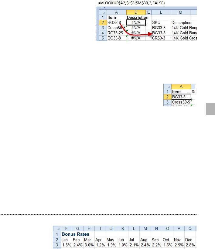
Problem: I’ve entered a VLOOKUP for January. I need to copy the formula across eleven additional col- umns.
Strategy: There are a few things you can do to make this process simpler:
●● Press F4 three times when entering the lookup value. This will change A2 to $A2. The single dollar sign ensures the lookup will always reach back to column A for the lookup value.
●● Press F4 once when entering the lookup table. This will change the lookup table to have four dollar signs, $P$4:$AB$227. Alternatively, name the lookup table first, then you won’t have to use dollar signs. See “Consider Naming the Lookup Table”
The big problem is the third argument. I find that I end up editing each copied formula to change to 2 to a
3, then a 4, then a 5, and so on.
I have two solutions for this.
●● Enter a temporary row with the numbers 2 through 13 stretching across the row. This row could be above the table you are trying to build. Then, instead of specifying 2 as the column to return, you can point to B1 and press F4 twice to change it to B$1.
Figure 406 Use a temporary column with the column numbers.
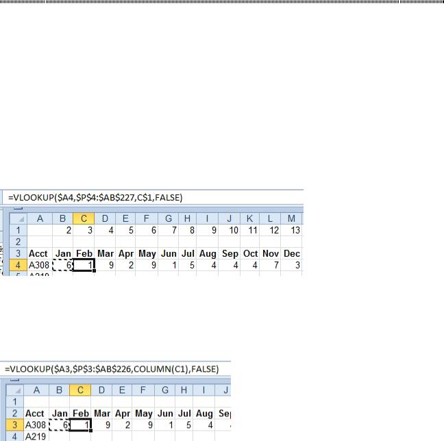
●● The other solution is to replace the ,2, with ,COLUMN(B1),. The COLUMN function returns the col- umn number of the given cell. Since B1 is in the second column, it will return a 2. I like to say that this is the world’s geekiest way of writing the number 2. However, the advantage is that when you copy this formula to the right, the reference inside the COLUMN function will automatically change to C1, which is in column 3. Using this method allows you to enter one formula without having the temporary values in row 1.
Figure 407 Use COLUMN(C1) to write a 3.
Additional Details: The second method will slow your VLOOKUPs down, as Excel has to calculate the COLUMN function in every row of your lookup table.
Alternate Strategy: You can speed up the VLOOKUPs if you add one column of MATCH functions and then use 12 columns of the incredibly speedy INDEX function. Before you can do this, though, you need to learn about these two incredibly arcane functions.
PART 2: CALCULATING WITH EXCEL |
|
165 |
|
|
|
|
INDEX SOUNDS LIKE AN INANE FUNCTION |
|
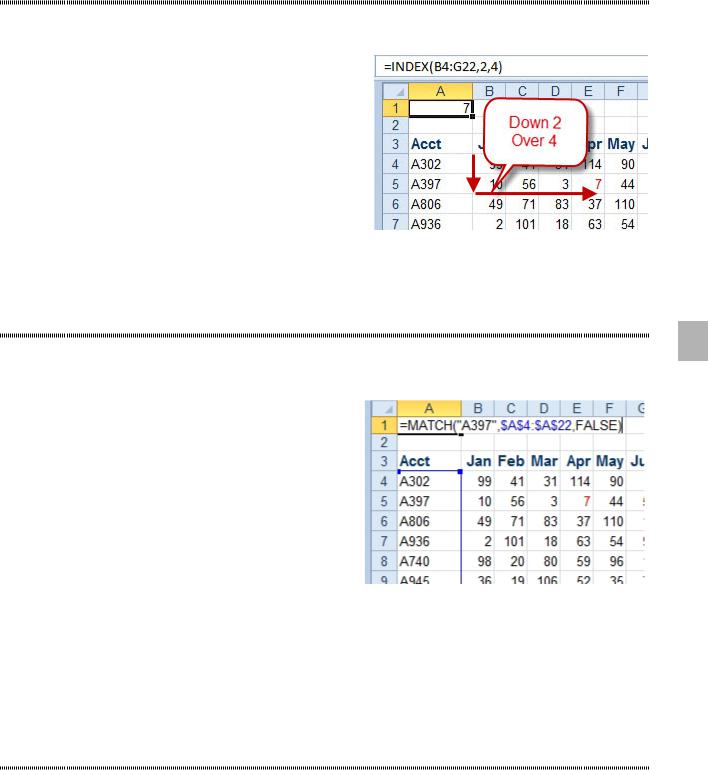
Problem: I was reading Excel Help for fun the other day and I read about a function called INDEX. Who in their right mind would ever use =INDEX(B4:G22,2,4) to point to cell F6?
Figure 408 The INDEX function seems useless.
Strategy: You will never use INDEX without using MATCH as either the second or third argument. Come back to INDEX after you see what MATCH does.
YOU ALREADY KNOW MATCH, REALLY!
2
Problem: The author of this book is jamming two functions that I have NEVER heard of on the same page. He is starting to hack me off.
Strategy: Really, if you know and love VLOOKUP, you already know MATCH. Let me compare and contrast:
●● The first argument is a lookup value just like VLOOKUP.
●● The lookup table is a single column, not a rectangular range.
●● You don’t have to specify a column number, so leave off the third argument.
●● The last argument could be FALSE just like VLOOKUP, although most people use zero in- stead of FALSE.
Figure 409 MATCH is a VLOOKUP in disguise.
So far, so good. It is just like a VLOOKUP.
The one difference that seems confusing... MATCH does not return a value from the table. MATCH tells you which row in the table contains the MATCH. I remember reading about this in Excel help and won- dering when I would ever have a manager call me up and ask, “Hey Bill, what ROW is that in?” Here is the trick: You will ALWAYS be entering your MATCH inside of an INDEX function. So, back to INDEX.
INDEX SOUNDS LIKE AN INANE FUNCTION - II
Strategy: The trick is to use INDEX to return a value. Use MATCH as the second and/or third argument to calculate which row or column to return on the fly.
The next four topics show how you can use MATCH with INDEX to solve some common problems.