

174 |
POWER EXCEL WITH MR EXCEL |
|
|
|
WATCH FOR DUPLICATES WHEN USING VLOOKUP |
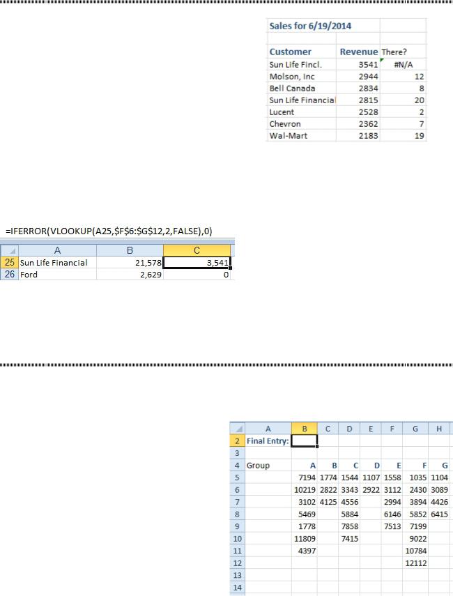
Problem: I used the VLOOKUP function to get sales from a second list into an original list, and then I received the next day’s sales in a file. When I use the MATCH function to find new customers, there is one new customer: Sun Life Fincl.
This is not really a new customer at all. Someone in the order entry department created a new customer instead of using the existing customer named Sun Life Financial. As a quick fix, you copy cell D9 and paste it in cell D6. This seems like a fine solution and resolves the #N/A error in F6
However, when I enter the VLOOKUP formula in column C
to get the current day’s sales, there are two rows that match Figure 428 Is this really a new customer?
Sun Life Financial..
Strategy: It’s important that you understand how VLOOKUP handles duplicates in the lookup list. The VLOOKUP function is not capable of handling the situation described here. When two rows match a VLOOKUP, the function will return the sales from the first row in the list. You will get the $3541, but you will not get the $2815.
Figure 429 VLOOKUP returns the first match that it finds.
If you are not absolutely sure that the customers in the lookup table are unique, you should not use
VLOOKUP. You could use a SUMIF function instead. See "Sum Records That Match a Criterion" on page 156 for details.
RETURN THE LAST ENTRY
Problem: Someone has logged some data. For each group, data starts in row 5 and continues down for some number of rows. There are a different number of data points in each column. I need to get the last entry in each column.
Strategy: There are multiple solutions to this problem. You could combine the unwieldy OFFSET with COUNT, but this topic will show you how to solve the problem using the approximate match version of VLOOKUP.
Flip back to Figure 376 and Figure 377 where you used the approximate match version of VLOOKUP to find a commission rate. The table had entries like 1000, 5000, 10000, and 20000. When someone had a sale of $12,345, the VLOOKUP would find the commission rate for the $10,000 level, because $10,000 was just less than the $12,345 that you were looking up.
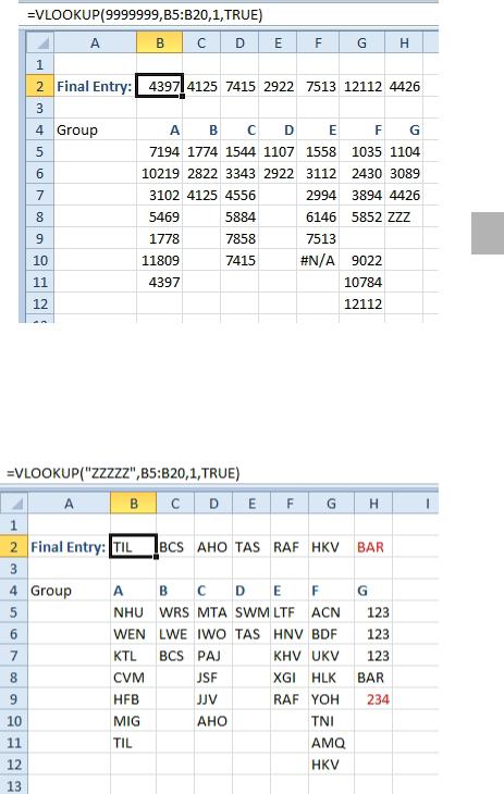
Figure 430 Return the last number in the column.
In this case, the data is not sorted nor should it be sorted. However, if you ask VLOOKUP to look for a re- ally large number, it will automatically return the last non-blank entry in the column!
PART 2: CALCULATING WITH EXCEL |
175 |
|
|
Some will suggest that you should use 9.99999999999999E+307 as the lookup value. This is the largest number possible in Excel. However, rather than type all of those characters, you can simply use a number that is larger than anyone would expect. For example, if you work for a company that has $1 Million in revenue per year, there is no way that the sales for one day would ever exceed $100K. You could safely search for 99999.
In the formula below, I held down the 9 key for a second and ended up searching for 9.9 million. It doesn’t matter exactly what you are searching for, just so long as it is larger than any possible number in the list.
Use =VLOOKUP(9999999,B5:B20,1,TRUE).
2
Figure 431 This VLOOKUP returns the last numeric value.
This is a really cool use of the rare version of VLOOKUP. As you can see in column G, the formula doesn’t get confused by blank cells. It will only return numeric values, so the errant ZZZ entry in H8 is ignored. The #N/A error in F10 is ignored.
If the entries in the column are text, then you would search for some text which will occur alphabetically after any text that you might expect. For example, search for “ZZZZZZ”.
Figure 432 Search for ZZZZZZ to return the last text entry.
Column H above illustrates a problem with this method. If the values can contain text or a number, the VLOOKUP will not work.
176 |
POWER EXCEL WITH MR EXCEL |
|
|
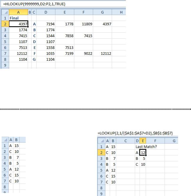
What if the data is turned sideways and you need to get the last value from each row? Use HLOOKUP instead of VLOOKUP.
Figure 433 Get the last entry from each row.
Additional Details: You do not have to put the ,TRUE at the end of any of these formulas. If you leave off the fourth argument, Excel assumes that you mean TRUE. However, since 99.9% of the VLOOKUPs in the world use FALSE at the end, I put the TRUE out there to help remind me that something unusual is happening with this formula.
RETURN THE LAST MATCHING VALUE
Problem: VLOOKUP returns the first match that it finds. I need to get the last match in the data. In this figure, I want to lookup A and find the 12 from row 5, since that is the latest data for A.
Figure 434 Find the last match for each letter.
Strategy: Use:
=LOOKUP(2,1/($A$1:$A$7=D2),$B$1:$B$7).
Figure 435 No one at your office will have a clue what you are doing.
First, LOOKUP is an ancient function that Excel includes for backwards compatibility with Quattro Pro.
It is a bizarre little function that takes a lookup value, a lookup vector, and a results vector. It always uses the Approximate Match version that you would get when using TRUE at the end of your VLOOKUP. Like the approximate match, LOOKUP expects the table to be sorted, but since you are using this formula to trick Excel, the table does not have to be sorted.
People end up using LOOKUP instead of VLOOKUP because LOOKUP works with arrays that VLOOK- UP won’t work with. Both this topic and the next topic show of the array-handling ability of LOOKUP.
This formula came from the MrExcel Message Board, originally posted to a MrExcel MVP named Fairwinds.
Let me explain the formula step by step, starting with A1:A7=D2. This comparison will produce a series of TRUE/FALSE values. In the figure above, you would end up with {TRUE; FALSE; FALSE; FALSE; TRUE; FALSE; FALSE}.
PART 2: CALCULATING WITH EXCEL |
177 |
|
|
Next, the formula divides that array into the number 1. Flip back to Figure 373 to see that Excel treats
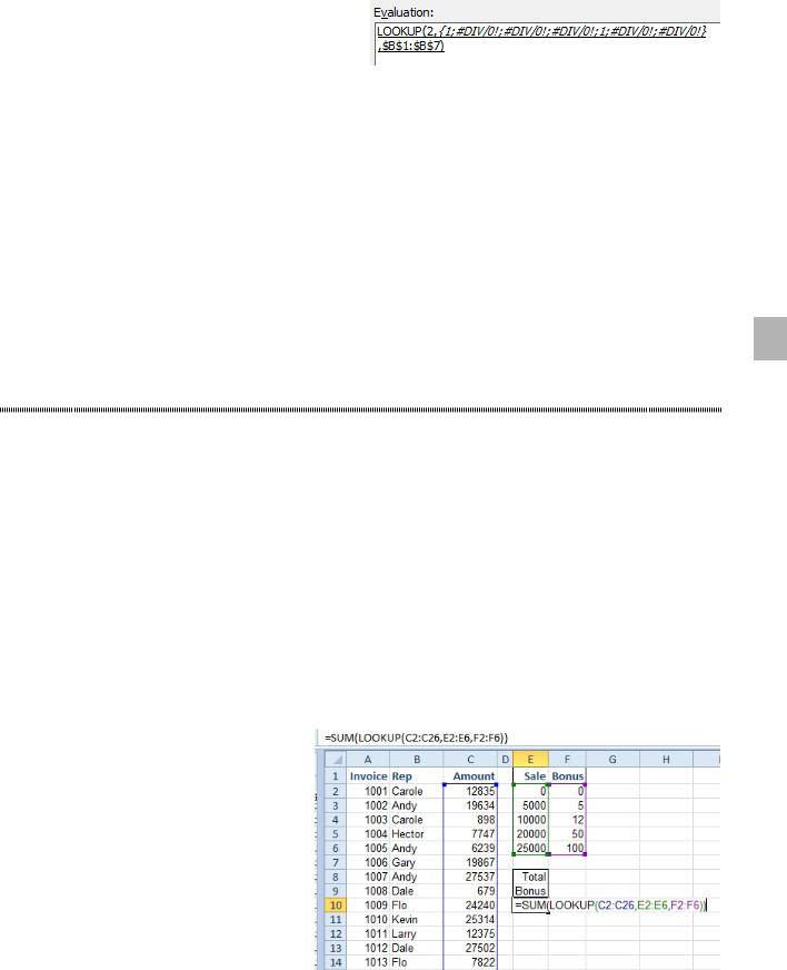
TRUE like 1 and FALSE like 0. Of course, 1/1 is 1. But 1/0 is a DIV/0 error. After doing the division, you have a series of values that are either 1 or #DIV/0!: {1; #DIV/0!; #DIV/0!; #DIV/0!; 1; #DIV/0!; #DIV/0!}.
Figure 436 From the Evaluate Formula dialog, after the fourth step.
If you flip back to Figure 431, you can see that the approximate VLOOKUP is ignoring text entries and error values. The same thing works here.
Also, in the last topic, there was a question if you should look for 9.99999999999999E+307 or simply 99999999. As you learned in the last topic, you just have to search for a number that is larger than any expected value. The logical test is either going to return 1 or #DIV/0!. There is no way that you will ever get anything larger than a 1 at this point of the formula. So, you can simply search for a 2.
When LOOKUP is searching for a 2 in {1; #DIV/0!; #DIV/0!; #DIV/0!; 1; #DIV/0!; #DIV/0!}, it can not find the 2. It thus uses the last numeric entry. In this case, it is the 1 that was calculated from cell A5. LOOK-
UP will return the fifth entry from the results vector. Since the results vector is B1:B7, Excel will return the 12 from cell B5.
Additional Details: The community of Excel aficionados at the MrExcel.com Message Board create some
of the wildest formulas that I’ve ever seen. I took a collection of these formulas and put them in my book, 2 Excel Gurus Gone Wild.
SUM ALL OF THE LOOKUPS
Problem: Are there any other arcane tricks with the old LOOKUP function that you can use to close out this string of topics on lookup?
Strategy: I am glad that you asked!
Say that you want to figure out the total bonus payments for the month so that you can accrue money to pay the bonus. You aren’t ready to pay the bonus yet, so you don’t have to do all the lookups. You just want one formula that does all of the lookups and totals the values.
Using SUM(VLOOKUP()) will not work, even if you use Ctrl+Shift+Enter to make it an array formula.
However, using SUM(LOOKUP()) with Ctrl+Shift+Enter will correctly do all the individual lookups and sum them.
Gotcha: As mentioned in the last topic, the LOOKUP command only does the approximate-match type of lookup, so this trick is likely only useful to the SCAIA (aka Scientists, Commission Accountants, and IRS Agents for those of you who have not been paying careful attention.)
Type the formula =SUM(LOOKUP(C2:C26,E2:E6,F2:F6)) but do not press Enter.
Figure 437 One formula does many lookups.