

166 |
POWER EXCEL WITH MR EXCEL |
|
|
|
VLOOKUP LEFT |
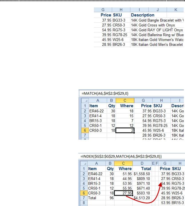
Problem: The lookup table is maintained by another department. They built it with the price to the left of the item number. Can I specify -1 as the third term of the VLOOKUP to indicate that I want a value to the left of the key field?
Figure 410 Lookup a value to the left of SKU.
Strategy: Unfortunately, the Excel team doesn’t offer the ability to VLOOKUP to the left of the key field. However, you can use MATCH to figure out which price to use.
Before you see how to solve this with MATCH and INDEX, the obvious solution would be to copy column G over to column J and then do a VLOOKUP. You are suspending reality here and assuming that you can’t move the price. Perhaps the data is coming in from a web query and is refreshed every five minutes?
The SKU’s are in H2:H29. They are not sorted, nor do they have to be. Each SKU occurs only once.
Look at the formula in C6. It is =MATCH(A6,$H$2:$H$29,0) which tells Excel to find CR-50 in the range of H2:H29. The final 0 indicates that you are looking for an exact match.
Look at the answer from the MATCH function. It says CR50-3 is in row 2, but you can see that CR50-3 is actually in H3 which is row 3 of the spreadsheet. This is an important distinction. MATCH returns the relative position of the item within the lookup range. The answer of 2 says that
CR50-3 is in the second cell of H2:H29.
Now that you know the position of the item within the lookup table, you can use the INDEX function to return the price.
You will specify the range of prices as the first argument of the INDEX function. The second argument specifies the row within the lookup table. When you have a singlecolumn lookup table, you do not have to specify the column in the third argument.
MATCH assumes you want column 1. The prices are in G2:G29. Use: =INDEX(G2:G29, MATCH(A6,$H$2:$H$29,0)).
Figure 411 MATCH locates CR50-3 in the lookup table.
Figure 412 Essentially a VLOOKUP Left.
PART 2: CALCULATING WITH EXCEL |
|
167 |
|
|
|
|
FAST MULTI-COLUMN VLOOKUP |
|
Problem: I have to do twelve columns of VLOOKUP. The lookup table is large. The data set is even larger.
It is taking forever to calculate.
VLOOKUP is an expensive function. It takes a lot of time to find the exact match in the lookup table.
Worse, consider one row of your table. Excel might have to search through a 200-row table to locate the
SKU when looking up the January value. When Excel goes to look up the February value, it must begin the search all over again. Yes, just a nanosecond earlier, Excel found A308 for January, but this is a new cell for February and Excel starts all over.
From a time perspective, MATCH and VLOOKUP take about as much time to calculate. INDEX takes a fraction of time. Excel can head directly to a particular row and grab the value.
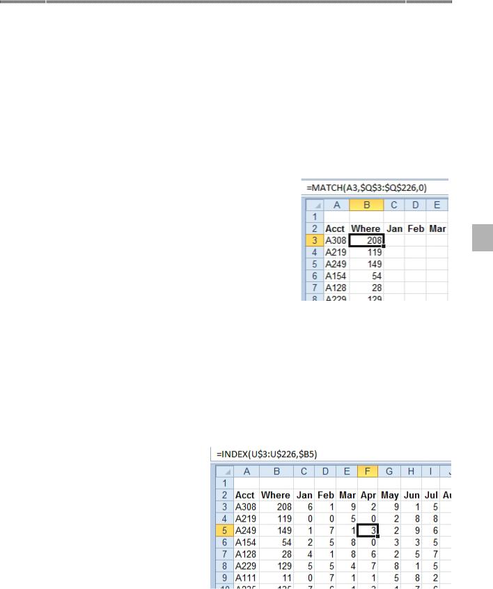
Strategy: Add a soon-to-be-hidden column called Where and put a MATCH formula there to figure out where the product is located. Once you know where the product, use 12 columns of INDEX to return the columns from the lookup table.
This figure shows the Where column. This column takes about as long to calculate as the January VLOOKUP would take.
Now that you have the MATCH running the Where column,
you can build an incredibly simple INDEX function. It is 2 interesting to consider the placement of dollar signs in this
formula.
Figure 413 Product A308 is found in the 208th row of the lookup table.
1.In cell C3, enter =INDEX(R$3:R$226,$B3). You are using $ before 3 and 226 to make sure that the lookup table is always pointing from row 3 to row 226. However, you are not using dollar signs be- fore column R. R3:R226 contains the January values. When you copy this formula to the right one cell, the lookup table shifts to the February column and points to S$3:S$226. The second argument of INDEX uses a single dollar sign before column B. This way, as you copy the formula, it is always pointing back to column B to get the row number of this product in the lookup table.
2.Copy C3 to D3:N3.
3.Select C3:N3.
4.Copy it down to all rows by double-clicking the fill handle in the lower right corner of N3.
5.Hide column B.
Figure 414 This table is 10 times faster than all VLOOKUPs.
The MATCH with INDEX solution shown here solves the whole problem of editing the third argument of the VLOOKUP for each column. Two simple formulas create the entire table. Plus, it runs much faster that using 12 columns of VLOOKUP.
I’ve met people who tell me that they have quit using VLOOKUP and rely entirely on MATCH and INDEX.
168 |
POWER EXCEL WITH MR EXCEL |
|
|
|
SPEED UP YOUR VLOOKUP |
Problem: I have to do thousands of VLOOKUPs and they are taking almost a minute every time that I recalculate the worksheet.
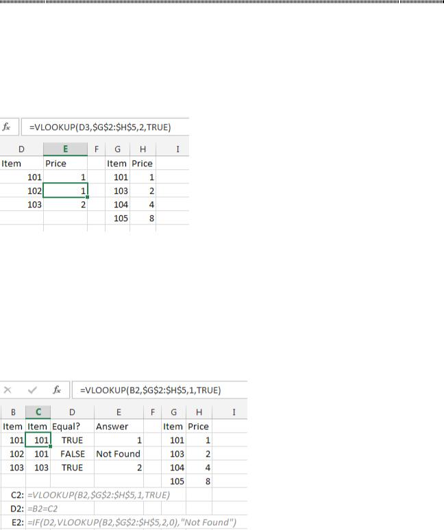
Strategy: Although it is counter-intuitive, two VLOOKUPs with the True argument will run over 100 times faster than the typical VLOOKUP. This is one time the lookup table will have to be sorted.
Gotcha: The reason you don’t use the True version of VLOOKUP is that it returns the wrong answer when the key field is not found. In the figure below, item 102 is missing from the lookup table. Instead of returning #N/A, the True version of VLOOKUP returns the answer from the next-lower item number. This is useless and dangerous!
Figure 415 The True version of VLOOKUP returns the wrong answer.
The foremost expert on Formula Speed is Charles Williams, creator of the FastExcelV3 utility. While most people would give up on the True version of VLOOKUP after seeing the above error, Charles realized that the True version of VLOOKUP is hundred times faster than the False version of VLOOKUP.
So, Charles thought up the idea of doing an extra VLOOKUP(A2,Table,1,True) before the real VLOOKUP. When you do a VLOOKUP to return the 1st item in the lookup table, you would normally get back the same value that you are looking up. In other words, =VLOOKUP(101,G2:H5,1,True) better return 101. If it returns something other than 101, then you know that the item is not found.
In the figure below, a formula in column C does a VLOOKUP to return column 1 from the lookup table. A formula in column D checks to see if B2=C2. If the result in D is True, then you know it is safe to do a VLOOKUP in column E. Otherwise, you should report that the value is Not Found.
Figure 416 Using a VLOOKUP in C2 to find if the result in E2 is correct or not.
You don’t have to do this in three columns as shown above. You can do a single formula with two VLOOK- UPs: =IF(D2=VLOOKUP(D2,$G$2:$H$5,1,TRUE),VLOOKUP(D2, $G$2:$H$5,2,TRUE),”N/A”).
If you see my live seminar, I probably showed how to use FastExcelV3 to time these formulas. I routinely take a 40-second recalc time and have it go to 0.2 seconds by using this formula. It is worth the hassle if you have a spreadsheet that is taking forever to calculate.
Note: This page contains just 1 of hundreds of amazing tricks from Charles Williams. Check out FastExcelV3 at http://tinyurl.com/fastexcel.
PART 2: CALCULATING WITH EXCEL |
169 |
|
|
RETURN THE NEXT LARGER VALUE IN A LOOKUP
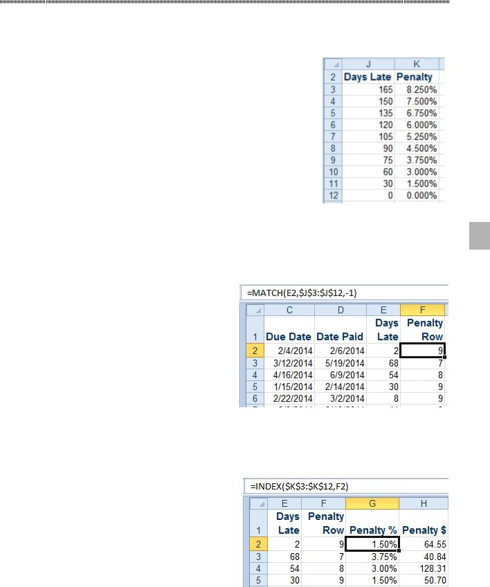
Problem: I am using a lookup table to calculate a late-payment penalty. As soon as a customer is 1 day late, they are charged the penalty for the first month. When they reach 31 days late, they pay for two months. After 60 days late, they are billed for half months.
Strategy: Earlier in “Nest IF Statements”, there was an example using the approximate version of VLOOKUP. This rare version would look for a match. When one is not found, it would return the row just smaller than the lookup value. In this case, you need the VLOOKUP to go the opposite way. VLOOKUP can not do that, but MATCH can.
Make sure that your penalty lookup table is sorted from high to low. (Hmmm, back in Figure 399, I should add rows for Credit Card Company Analysts and IRS Agents.)
Figure 417 Another rarity: the lookup table sorted descending.
You will see this calculation take shape after many intermediate steps. In real life, you could do all of these |
2 |
|
|
steps in a single formula. |
|
Calculate a Penalty Row in F2 with =MATCH(E2,$J$3:$J$12,-1). |
|
Figure 418 Find the row with the appropriate penalty.
Take a look at the results of that formula. In row 5, the payment is 30 days late. There is an exact match in Figure 417 for 30 days late, so the formula returns the exact match. However, in rows 2 through 4, there is no exact match. Because the third argument of MATCH is -1, Excel is returning the result from the next higher row in the table. The 68 days late in F3 is matched to the 75 day penalty in row 7 of the table.
Figure 419 Use INDEX to return the Penalty % from the table.
This is a third example of something that you can do with MATCH and INDEX that you can not do with a regular VLOOKUP.