

44 |
POWER EXCEL WITH MR EXCEL |
|
|
Additional Details: A great April Fools day trick is to add the custom list of Jan, Marcia, Cindy, Bobby, Greg, Peter as a custom list.
PUT DATE & TIME IN A CELL
Problem: I need to enter the current date, current time, or current date and time in a cell. I don’t want to use NOW() or TODAY(), because those values will change over time. I want to lock in the current date or time.
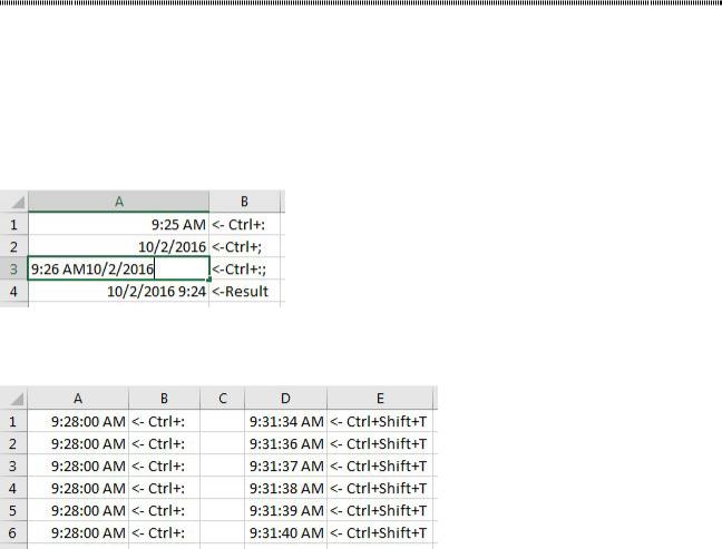
Strategy: Ctrl+: enters the current time. That should be easy to remember, since 9:26 includes a colon. To enter the current date, use the same keys, but don’t press shift. So, Ctrl+; puts in the current date.
What if you need both Date and Time? I learned this trick from Bob in Oklahoma City. Press Ctrl+: and then press Ctrl+;. Excel will show you the seemingly useless 9:26AM10/2/2016. When you press Enter,
Excel will convert it to a real date and time as shown in row 4 below.
Figure 94 Use Ctrl+: or Ctrl+; to apply a date or time stamp.
Gotcha: The Ctrl+: enters hours and minutes, but not seconds. If you enter Ctrl+: each second, 60 entries will be the same.
Figure 95 Ctrl+: does not provide seconds.
Alternate Strategy: Use a short macro stored in your Personal Macro Workbook and assign that macro to Ctrl+Shift+T. The macro can provide a time stamp that includes seconds.
First, make sure you have a Personal Macro Workbook. See "Create a Personal Macro Workbook" on page 64.
Switch over to VBA using Alt+F11. Display the Project Explorer using Ctrl+R. Open the Modules for Per- sonal and type this short macro:
Sub TimeStampSeconds() ActiveCell.Value = Time
End Sub
Use Alt+Q to return to Excel. Press Alt+F8 to display the list of macros. Click once on TimeStampSeconds and click Options. Click in to the Shortcut key field and type Shift+T. You’ve now assigned the macro to Ctrl+Shift+T.
Close Excel. You will get a message asking if you want to save the changes to Personal. Be sure to answer Yes.
Alternate Strategy: If you want to create a Date & Time stamp that is accurate to the second, use this macro instead:
Sub DateTimeStampSeconds() ActiveCell.Value = Date + Time
End Sub
PART 1: THE EXCEL ENVIRONMENT |
|
45 |
|
|
|
|
USE EXCEL AS A WORD PROCESSOR |
|
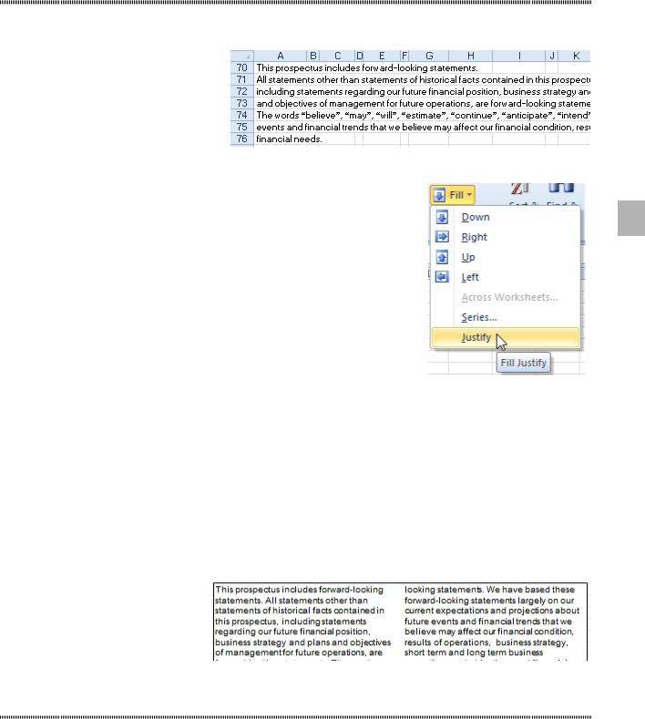
Problem: I need to type some notes at the bottom of a report. How can I make the words fill each line as if I had typed them in Word?
Figure 96 This paragraph needs to fit in A:G.
Strategy: You can use Fill, Justify. Follow these steps:
1. To have the words fill columns A through G, select a range
such as A70:G85. Include enough extra blank rows in the se- 1 lection to handle the text after word wrapping.
2. Select Home, Fill dropdown, Justify. (The Fill dropdown now appears in the Editing group of the Home tab. It often ap- pears as a blue down-arrow icon.)
Results: Excel will rearrange the text to fill each row.
Gotcha: If you have a few words in bold in one cell, this formatting will be lost.
Gotcha: If you later change the widths of columns A:G, you will have to use the Justify command again to force the data to fit.
Figure 97 Select Fill Justify.
Gotcha: Do not use this method if any of your cells contain more than 255 characters. Excel will silently truncate those cells to 255 characters without any notice!
Alternate Strategy: You can also use a text box to solve this problem. You simply click the Text box icon on the Insert tab, draw a text box to fill columns A through G, and paste your text into the text box. You can then format the text box to hide its border: Select the text box and on the Drawing Tools Format tab, select Shape Outline, None.
Additional Details: Starting in Excel 2007, you can give a text box multiple columns. To do so, you select the text box. On the Drawing Tools Format tab, you click the dialog launcher icon in the bottom-right cor- ner of the Shape Styles group to display the Format Shape dialog. In the left pane, you choose Text Box. Then you click on Columns and specify two columns, with separation between them of 0.1”.
Figure 98 Textboxes support multiple columns.
ADD EXCEL TO WORD
Problem: My co-worker is working on a report in Word. I need to add a table and chart to Word. I hate Word.
46 |
|
|
POWER EXCEL WITH MR EXCEL |
|
|
|
|
|
|
Strategy: You can use the full power of Excel |
|
|
|
in Word. While you are typing the document, |
|
|
|
you can put all of the Excel ribbon tabs in the |
|
|
|
Word ribbon. Follow these steps: |
|
|
|
1. |
Place the insertion point where the ta- |
|
|
2. |
ble should start. |
|
|
Select Insert, Object. Word will display |
|
|
|
3. |
the Object dialog box. |
|
|
Choose Microsoft Excel Worksheet. |
|
|
|
|
Click OK. You now have Excel ribbon |
|
|
4. |
tabs at the top of Word! |
|
|
Build your worksheet in the frame. You |
|
|
|
|
can use the resize handles in the corner |
|
|
|
of the frame to make the worksheet as |
|
|
5. |
wide and tall as necessary. |
|
|
Consider using View, Show, and un- |
|
|
|
|
check Gridlines. This will hide the grid- |
|
|
|
lines when the worksheet is embedded |
|
|
6. |
in Word. |
|
|
Click outside the spreadsheet frame. |
|
|
|
|
The worksheet appears in Word. |
|
|
Additional Details: It seems bizarre, but if |
|
|
|
you need to put a Word paragraph in Excel, |
|
Figure 99 If you have to work in Word, it is better to |
you can use the same trick in Excel. Choose |
||
have Excel. |
Insert, Object, Microsoft Word. |
||
USE HYPERLINKS TO CREATE AN OPENING MENU FOR A WORKBOOK
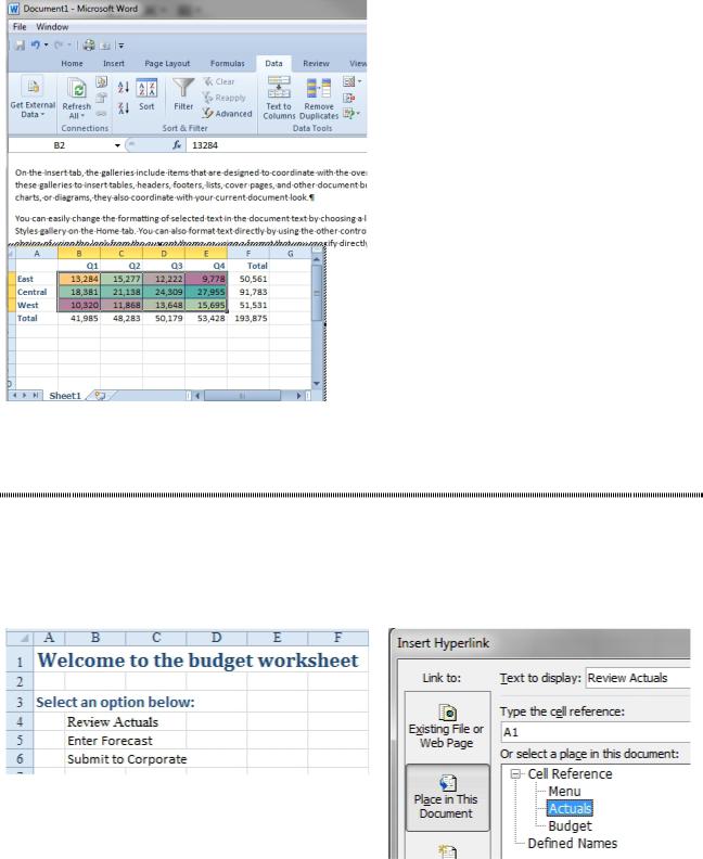
Problem: I have designed a budget workbook that has various worksheets. Managers throughout the company need to use it, but some of the managers are not entirely comfortable with Excel. A navigation tool would help them get through the worksheet.
Strategy: You can make your first worksheet a menu with hyperlinks. Here’s how:
1. Insert an opening worksheet called Menu. Add an entry for each section of the workbook.
Figure 100 Column B will become clickable hyper-
links.
2. Select cell B4 and then select Insert, Hyperlink or press Ctrl+K.
3. In the Insert Hyperlink dialog, choose Place In
This Document from the left icons.
4. Select the correct worksheet. Verify the cell ad- dress of A1.
5.Optionally, click the ScreenTip button and provide friendly text that will appear when someone hov- ers over the link.
Gotcha: If you don’t provide ScreenTip text, Excel will display a distracting ToolTip.
Results: The cell becomes a clickable hyperlink. Clicking on the link will take the manager to the Actuals worksheet.
PART 1: THE EXCEL ENVIRONMENT |
47 |
|
|
Additional Details: Be sure to provide a hyperlink on the Actuals worksheet to take the manager back |
|
to the menu |
|
Additional Details: It is tricky to select a hyperlinked cell. One method: Click on the hyperlink and hold the mouse button for two seconds. When the hand icon changes to a plus icon, let go of the mouse button.
To edit an existing hyperlink, you use the Insert, Hyperlink command again or right-click the cell and choose Edit Hyperlink.
See Also: "Remove Hyperlinks Automatically Inserted by Excel" on page 505.
|
SPELL CHECK A REGION |
|
|
|
|
|
|
Problem: I want to spell check the notes at the bottom of a report, but I don’t want to spell check the cus- |
|
||
tomer names in the report. How can I accomplish this? |
|
||
Strategy: You can select the region to be spell checked and then choose Review, Spelling. (Or press F7, |
|
||
the Spelling shortcut key). |
1 |
||
|
|
|
|
|
|
|
|
Figure 102 Select cells before invoking the Spelling command..
Results: Excel will spell check just the selected cells.
Gotcha: If you indicate to spell check a single cell, Excel will expand your selection to the entire worksheet. To get around this problem, you can select the desired cell and any one adjacent cell. When you have two or more cells selected, Excel will check only the selection.
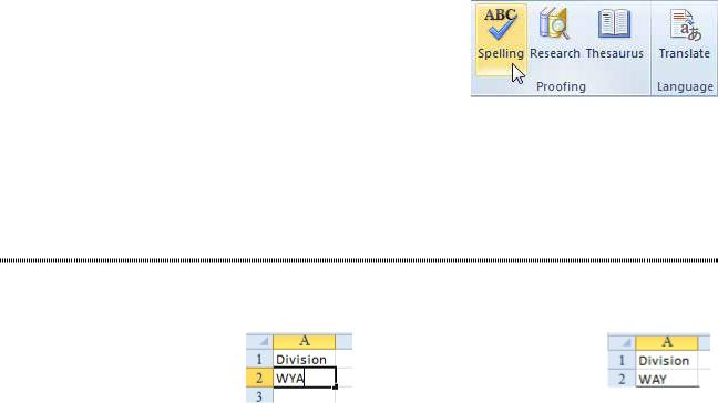
STOP EXCEL FROM AUTOCORRECTING CERTAIN WORDS
Problem: Every time I type the name of my WYA Division, Excel changes “WYA” to “WAY,”. It is impos- sible to type WYA without entering it as a formula: =”W”&”Y”&”A”.
Figure 103 WYA until…
Strategy: To help correct common mis-typings, Excel has a large list of words that are automatically replaced as you type. This is a good feature, unless you routinely have to type one of the words that Excel thinks is wrong. Luckily, you can edit this list rather than turning it off. Here’s how:
1. Select File, Options, Proofing, AutoCorrect Options or Alt+T+A.
2. On the AutoCorrect dialog, go to the AutoCorrect tab.
3. Scroll down the Replace Text as You Type section until you find the entry for replacing WYA with WAY. Select that line and click Delete.