3.8 · Spatial Characteristics of Secondary Electrons

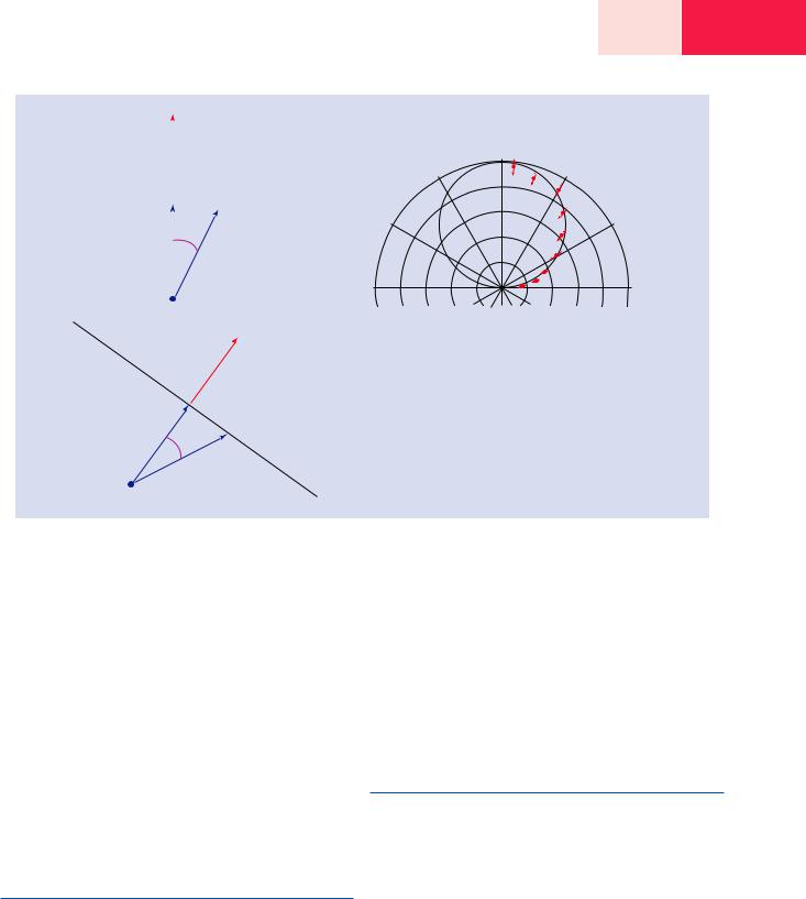
. Fig. 3.7  a Dependence of the secondary electron escape path length on the angle relative to the surface normal. The probability of escape decreases as this path length increases. b Angular distribution of secondary electrons as a function of the angle relative to the surface

normal as simulated by Monte Carlo calculations (Koshikawa and Shimizu 1974) compared to a cosine function. c The escape path length situation of .  Fig. 3.7a for the case of a tilted specimen. A cosine dependence relative to the surface normal is again predicted

secondary electrons is expected to follow a cosine relation with the emergence angle relative to the local surface normal. Behavior close to a cosine relation is seen in the Monte Carlo simulation of Koshikawa and Shimizu (1974) in

.  Fig. 3.7b.

Even when the surface is highly tilted relative to the beam, the escape path length situation for a secondary electron generated below the surface is identical to the case for normal beam incidence, as shown in .  Fig. 3.7c. Thus, the secondary electron trajectories follow a cosine distribution relative to the local surface normal regardless of the specimen tilt.

3.7\ Secondary Electron Yield Versus Beam

Energy

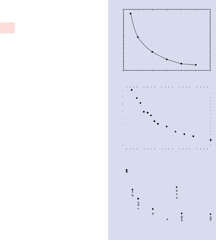
The secondary electron coefficient increases as the incident beam energy decreases, as shown for copper in .  Fig. 3.8a for the conventional beam energy range (5 keV ≤E0 ≤30 keV) and in .  Fig. 3.8b for the low beam energy range (E0 < 5 keV). This behavior arises from two principal factors: (1) as the beam electron energy decreases, the rate of energy loss, dE/ds, increases so that more energy is deposited per unit of beam electron path length leading to more secondary electron generation per unit of path length; and (2) the range of the beam

electrons is reduced so more of that energy is deposited and more secondary electrons are generated in the near surface region from which secondary electrons can escape. This is a general behavior found across the Periodic Table, as seen in the plots for C, Al, Cu, Ag, and Au in .  Fig. 3.8c.

3.8\ Spatial Characteristics of Secondary

Electrons

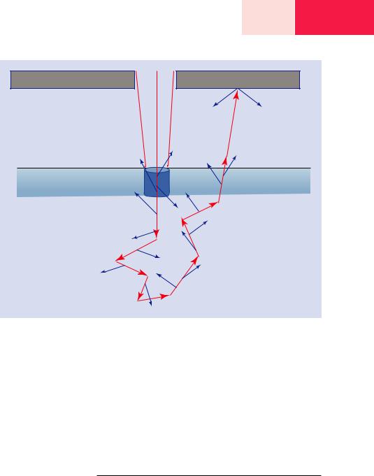
As the beam electrons enter the sample surface, they begin to generate secondary electrons in a cylindrical volume whose cross section is defined by the footprint of the beam on the entrance surface and whose height is the escape depth of the SE, as shown schematically in .  Fig. 3.9 These entrance surface SE, designated the SE1 class, preserve the lateral spatial resolution information defined by the dimensions of the focused beam and are similarly sensitive to the properties of the near surface region due to the shallow scale of their origin. As the beam electrons move deeper into the solid, they continue to generate SE, but these SE rapidly lose their small initial kinetic energy and are completely reabsorbed within an extremely short range. However, for those beam electrons that subsequently undergo enough scattering to return to the entrance surface to emerge as backscattered electrons (or reach any

36\ Chapter 3 · Secondary Electrons

. Fig. 3.8  a Behavior of the secondary electron coefficient as a function of incident beam energy for the conventional beam energy range, E0 = 5–30 keV (Data of Moncrieff and Barker (1976)). b Behavior of the secondary electron coefficient as a function of incident beam energy for the low beam energy range, E0 < 5 keV (data) (Data of Bongeler et al. (1993)). c Dependence of the secondary electron coefficient

3 on incident beam energy for C, Al, Cu, Ag, and Au (Reimer and Tolkamp 1980)

a

Secondary coefficientelectron

b

Secondary coefficientelectron

c

Secondary coefficientelectron

Secondary electron yield vs. beam energy for copper

0.8

Moncrieff and Barker (1976)

0.7

0.6

0.5

0.4

Beam energy (keV)

References

. Fig. 3.9  Schematic diagram showing the origins of the SE1, SE2, and SE3 classes of secondary electrons. The SE1 class carries the lateral and near-surface spatial information defined by the incident beam, while the SE2 and SE3 classes actually carry backscattered electron information. The blue rectangle represents the escape depth for SE, and the cylinder represents the volume from which the SE1 escape

other surface for specimens with more complex topography than a simple flat bulk target), the SE that they continue to generate as they approach the surface region will escape and add to the total secondary electron production, as shown in .  Fig. 3.9. This class of SE is designated SE2 and they are indistinguishable from the SE1 class based on their energy and angular distributions. However, because of their origin from the backscattered electrons, the SE2 class actually carries the degraded lateral spatial distribution of the BSE: because the relative number of SE2 rises and falls with backscattering, the SE2 signal actually carries the same information as BSE. That is, the relative number of the SE2 scales with whatever specimen property affects electron backscattering. Finally, the BSE that leave the specimen are energetic, and after traveling millimeters to centimeters in the specimen chamber, these BSE are likely to hit other metal surfaces (objective lens polepiece, chamber walls, stage components, etc.), generating a third set of secondary electrons designated SE3. The SE3 class again represents BSE information, including the degraded spatial resolution, not true SE1 information and resolution. The SE1 and SE2 classes represent an inherent property of a material, while the SE3 class depends on the details of the SEM specimen chamber. Peters (1984) measured the three secondary electron classes for thin and thick gold targets to estimate the relative populations of each class:

Incident beam footprint, high resolution, SE1 (9 %) BSE generated at specimen, low resolution, SE2 (28 %)

BSE generated remotely on lens, chamber walls, SE3 (61 %)

A small SE contribution designated the SE4 class arises from pre-specimen instrumental sources such as the final aperture

(2 %) that depends in detail on the instrument construction (apertures, magnetic fields, etc.). These measurements show

that for gold the sum of the SE2 and SE3 classes which actually carry BSE is nearly ten times larger than the high resolution, high surface sensitivity SE1 component. These three classes of secondary electrons influence SEM images of compositional structures and topographic structures in complex ways. The appearance of the SE image of a structure depends on the details of the secondary electron emission and the properties of the secondary electron detector used to capture the signal, as discussed in detail in the image formation module.

References

Bongeler R, Golla U, Kussens M, Reimer L, Schendler B, Senkel R, Spranck M (1993) Electron-specimen interactions in low voltage scanning electron microscopy. Scanning 15:1

Joy D (2012) Can be found in chapter 3 on SpringerLink: http://link. springer.com/chapter/10.1007/978-1-4939-6676-9_3

Kanaya K, Ono S (1984) Interaction of electron beam with the target in scanning electron microscope. In: Kyser DF, Niedrig H, Newbury DE, Shimizu R (eds) Electron interactions with solids. SEM, Inc, Chicago, pp 69–98

Koshikawa T, Shimizu R (1973) Secondary electron and backscattering measurements for polycrystalline copper with a retarding-field analyser. J Phys D Appl Phys 6:1369

Koshikawa T, Shimizu R (1974) A Monte Carlo calculation of low-energy secondary electron emission from metals. J Phys D Appl Phys 7:1303 Peters K-R (1984) Generation, collection and properties of an SE-I enriched signal suitable for high resolution SEM on bulk specimens.

In: Kyser DF, Niedrig H, Newbury DE, Shimizu R (eds) Electron beam interactions with solids. SEM, Inc, AMF O’Hare, p 363

Moncrieff DA, Barker PR (1976) Secondary electron emission in the scanning electron microscope. Scanning 1:195

Reimer L, Tolkamp C (1980) Measuring the backscattering coefficient and secondary electron yield inside a scanning electron microscope. Scanning 3:35