1.4 · Simulating the Effects of Elastic Scattering: Monte Carlo Calculations

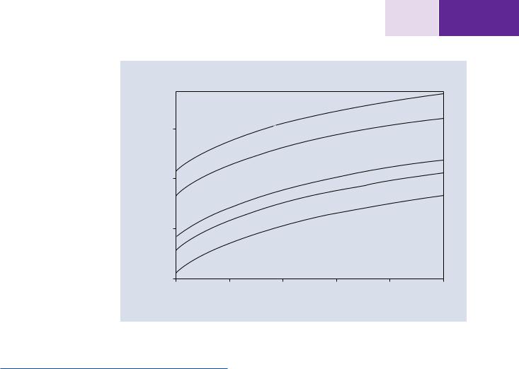
. Fig. 1.4  Elastic mean free path as a function of electron kinetic energy for various elements

Elastic mean free path (nm)

10

1

0.1

0.01

5

Elastic scattering mean free path (f0 = 2°)

C

Al

Cu

Ag

Au

1.4\ Simulating the Effects of Elastic

Scattering: Monte Carlo Calculations

Inelastic scattering sets a limit on the total distance traveled by the beam electron. The Bethe range is an estimate of this distance and can be found by integrating the Bethe continuous energy loss expression from the incident beam energy E0 down to a low energy limit, for example, 2 keV. Estimating the effects of elastic scattering on the beam electrons is much more complicated. Any individual elastic scattering event can result in a scattering angle within a broad range from a threshold of a fraction of a degree up to 180°, with small scattering angles much more likely than very large values and an average value typically in the range 5–10°. Moreover, the electron scattered by the atom through an angle ϕ in

.  Fig. 1.3a at point P1 can actually follow any path along the surface of the three-dimensional scattering cone shown in

.  Fig. 1.3b and can land anywhere in the circumference of the base of the scattering cone (i.e., the azimuthal angle in the base of the cone ranges from 0 to 360° with equal probability), resulting in a three-dimensional path. The length of the trajectory along the surface of the scattering cone depends on the frequency of elastic events with distance traveled and can be estimated from Eq. 1.3a for the elastic

scattering mean free path, λelastic. The next elastic scattering event P2 causes the electron to deviate in a new direction, as

shown in .  Fig. 1.3c, creating an increasingly complex path. Because of the random component of scattering at each of many steps, this complex behavior cannot be adequately described by an algebraic expression like the Bethe continuous energy loss equation. Instead, a stepwise simulation of the electron's behavior must be constructed that incorporates inelastic and elastic scattering. Several simplifications are introduced to create a practical “Monte Carlo electron trajectory simulation”:

\1.\ All of the angular deviation of the beam electron is ascribed to elastic scattering. A mathematical model for elastic scattering is applied that utilizes a random number (hence the name “Monte Carlo” from the supposed randomness of gambling) to select a properly weighted value of the elastic scattering angle out of the possible range (from a threshold value of approximately 1° to a maximum of 180°). A second random number is used to select the azimuthal angle in the base of the scattering cone in .  Fig. 1.1c.

\2.\ The distance between elastic scattering events, s, which lies on the surface of the scattering cone in .  Fig. 1.3b, is calculated from the elastic mean free path, Eq. 1.3b.

\3.\ Inelastic scattering is calculated with the Bethe continuous energy loss expression, Eq. 1.1b. The specific energy loss, E, along the path, s, in the surface of the scattering cone, .  Fig. 1.3b, is calculated with the Bethe continuous energy loss expression: E = (dE/ds)*s

Given a specific set of these parameters, the Monte Carlo elec- 1 tron trajectory simulation utilizes geometrical expressions to calculate the successive series of locations P1, P2, P3, etc., successively determining the coordinate locations (x, y, z) that the energetic electron follows within the solid. At each location P, the newly depreciated energy of the electron is known, and after the next elastic scattering angle is calculated, the new velocity vector components vx, vy, vz are determined to transport the electron to the next location. A trajectory ends when either the electron energy falls below a threshold of interest (e.g., 1 keV), or else the path takes it outside the geometric bounds of the specimen, which is determined by comparing the current location (x, y, z) with the specimen boundaries. The capability of simulating electron beam interactions in specimens with complex geometrical shapes is one of the major strengths of the

Monte Carlo electron trajectory simulation method.

Monte Carlo electron trajectory simulation can provide visual depictions as well as numerical results of the beam–specimen interaction, creating a powerful instructional tool for studying this complex phenomenon. Several powerful Monte Carlo simulations appropriate for SEM and X-ray microanalysis applications are available as free resources:

CASINO [7http://www.gel.usherbrooke.ca/casino/What.html] Joy Monte Carlo [7http://web.utk.edu/~srcutk/htm/

simulati.htm]

NIST DTSA-II [7http://www.cstl.nist.gov/div837/837.02/ epq/dtsa2/index.html]

While the static images of Monte Carlo simulations presented below are useful instructional aids, readers are encouraged to perform their own simulations to become familiar with this powerful tool, which in more elaborate implementations is an important aid in understanding critical aspects of SEM imaging.

1.4.1\ What Do Individual Monte Carlo

Trajectories Look Like?

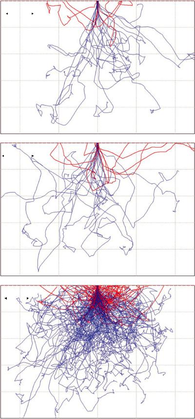
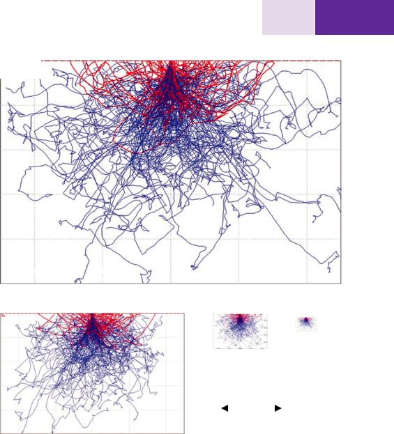
Perform a Monte Carlo simulation (CASINO simulation) for copper with a beam energy of 20 keV and a tilt of 0° (beam perpendicular to the surface) for a small number of trajectories, for example, 25. .  Figure 1.5a, b show two simulations of 25 trajectories each. The trajectories are actually determined in three dimensions (x-y-z, where x-y defines the surface plane and z is perpendicular to the surface) but for plotting are rendered in two dimensions (x-z), with the third

dimension y projected onto the x-z plane. (An example of the true three-dimensional trajectories, simulated with the Joy Monte Carlo, is shown in .  Fig. 1.6, in which a small number of trajectories (to minimize overlap) have been rendered as an anaglyph stereo representation with the convention left eye = red filter. Inspection of this simulation shows the y motion of the electrons in and out of the x-z plane.) The stochastic nature of the interaction imposed by the nature of elastic scattering is readily apparent in the great variation among the individual trajectories seen in .  Fig. 1.5a, b. It quickly becomes clear that individual beam electrons follow a huge range of paths and simulating a small number of trajectories does not provide an adequate view of the electron beam specimen interaction.

1.4.2\ Monte Carlo Simulation To Visualize

the Electron Interaction Volume

To capture a reasonable picture representation of the electron interaction volume, which is the region of the specimen in which the beam electrons travel and deposit energy, it is necessary to calculate many more trajectories. .  Figure 1.5c shows the simulation for copper, E0 = 20 keV at 0° tilt extended to 500 trajectories, which reveals the full extent of the electron interaction volume. Beyond a few hundred trajectories, superimposing the three-dimensional trajectories to create a two-dimensional representation reaches diminishing returns due to overlap of the plotted lines. While simulating 500 trajectories provides a reasonable qualitative view of the electron interaction volume, Monte Carlo calculations of numerical properties of the interaction volume and related processes, such as electron backscattering (discussed in the backscattered electron module), are subject to statistically predictable variations because of the use of random numbers to select the elastic scattering parameters. Variance in repeated simulations of the same starting conditions is related to the number of trajectories and can be described with the properties of the Gaussian (normal) distribution. Thus the precision, p, of the calculation of a parameter of the interaction is related to the total number of simulated trajectories, n, and the fraction, f, of those trajectories that produce the effect of interest (e.g., backscattering):

1

Energy (keV) 20

Tilt/TOA 0

Number 35

Select

500 nm

Repeat

. Fig. 1.6  Three-dimensional representation of a Monte Carlo simulation (Cu, 20 keV, 0° tilt) using the anaglyph stereo method (left eye = red filter) (Joy Monte Carlo)

1.4.3\ Using the Monte Carlo Electron

Trajectory Simulation to Study

the Interaction Volume

What Are the Main Features of the Beam Electron Interaction Volume?

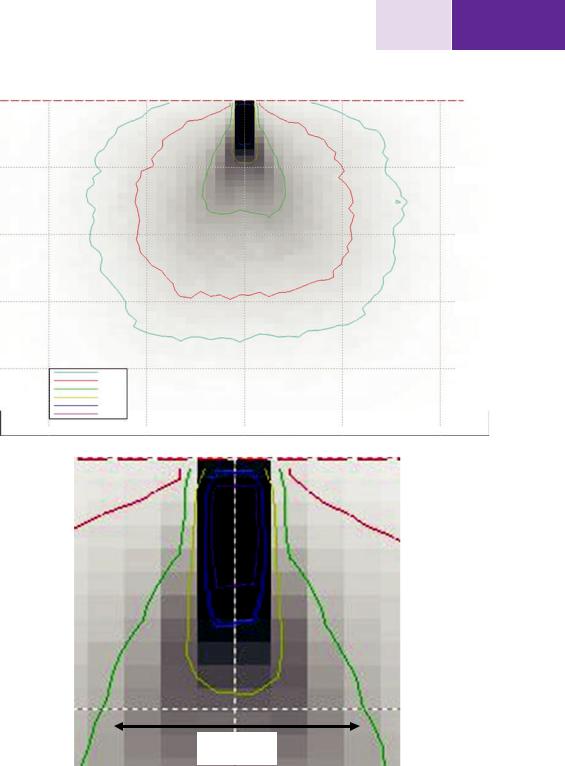
In .  Fig. 1.5c, the beam electron interaction volume is seen to be a very complex structure with dimensions extending over hundreds to thousands of nanometers from the beam impact point, depending on target material and the beam energy. At 0° tilt, the interaction volume is rotationally symmetric around the beam. While the electron trajectories provide a strong visual representation of the interaction volume, more informative numerical information is needed. The Monte Carlo simulation can provide detailed information on many aspects of the electron beam–specimen interaction. The color-encoding of the energy deposited along each trajectory, as implemented in the Joy Monte Carlo shown in .  Fig. 1.11, creates a view that reveals the general three-dimensional complexity of energy deposition within the interaction volume. The CASINO Monte Carlo provides an even more detailed view of energy deposition, as shown in .  Fig. 1.7. The energy deposition per unit volume is greatest just under the beam impact location and rapidly falls off as the periphery of the interaction volume is approached. This calculation reveals that a small cylindrical volume under the beam impact point, shown in more detail in .  Fig. 1.7b, receives half of the total energy deposited by the beam in the specimen (that is, the volume within the 50% contour), with the

balance of the energy deposited in a strongly non-linear fashion in the much larger portion of the interaction volume.

How Does the Interaction Volume Change with Composition?

.  Figure 1.8 shows the interaction volume in various targets, C, Si, Cu, Ag, and Au, at fixed beam energy, E0 = 20 keV, and 0° tilt. As the atomic number of the target increases, the linear dimensions of the interaction volume decrease. The form also changes from pear-shaped with a dense conical region below the beam impact for low atomic number targets to a more hemispherical shape for high atomic number targets.

kNote the dramatic change of scale

Approximately 12 gold atoms were encountered within the footprint of a 1-nm diameter at the surface. Without considering the effects of elastic scattering, the Bethe range for Au at an incident beam energy of 20 keV limited the penetration of the beam to approximately 1200 nm and a cylindrical volume of approximately 940 nm3, containing approximately 5.6 × 104 Au atoms. The effect of elastic scattering is to create a three-dimensional hemispherical interaction volume with a radius of approximately 600 nm and a volume of 4.5 × 108 nm3, containing 2.7 × 1010 Au atoms, an increase of nine orders-of-magnitude over the number of atoms encountered in the initial beam footprint on the surface.

How Does the Interaction Volume Change with Incident Beam Energy?

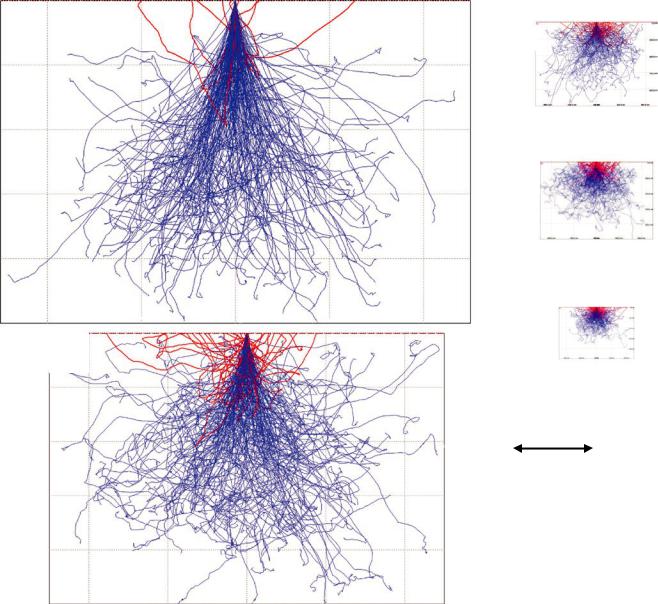
.  Figure 1.9 shows the interaction volume for copper at 0° tilt over a range of incident beam energy from 5 to 30 keV. The shape of the interaction volume is relatively independent of beam energy, but the size increases rapidly as the incident beam energy increases.

How Does the Interaction Volume Change with Specimen Tilt?

.  Figure 1.10 shows the interaction volume for copper at an incident beam energy of 20 keV and a series of tilt angles. As the tilt angle increases so that the beam approaches the surface at a progressively more shallow angle, the shape of the interaction volume changes significantly. At 0° tilt, the interaction volume is rotationally symmetric around the beam, but as the tilt angle increases the interaction volume becomes asymmetric, with the dense portion of the distribution shifting progressively away from the beam impact point. The maximum penetration of the beam is reduced as the tilt angle increases.

1.4 · Simulating the Effects of Elastic Scattering: Monte Carlo Calculations

91

0.0nm

206.3nm

412.6nm

618.9nm

825.2nm

1.4 · Simulating the Effects of Elastic Scattering: Monte Carlo Calculations

. Fig. 1.9  Monte Carlo simula-

tions for Cu, 0° tilt, incident beam 30 keV energies 5, 10, 20, and 30 keV

(CASINO Monte Carlo simulation)

-1260.0 nm -630.0 nm 0.0 nm 630.0 nm

10 keV

111

0.0nm

432.6 nm

865.2 nm

1297.8 nm

1730.4 nm

1260.0 nm

5 keV