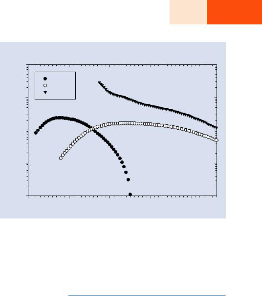
. Fig. 4.8  Product of the ionization cross section, the fluorescence yield, and the relative weights of lines for the most intense member of the K-, L-, and M-shells for E0 = 30 keV

Product of ionization cross section, relative transition probability and fluorescence yield

Atomic number (Z)

strong differences in the relative abundance of the X-rays produced by different elements. This plot also reveals that over certain atomic number ranges, two different atomic shells can be excited for each element, for example, K and L for Z = 16 to Z = 50, and L and M for Z = 36 to Z = 92. For lower values of E0, these atomic number ranges will be diminished.

X-Ray Intensity Emitted from Thick, Solid Specimens

A thick specimen is one with sufficient thickness so that it contains the full electron interaction volume, which generally requires a thickness of at least a few micrometers for most choices of composition and incident beam energy. Within the interaction volume, the complete range of elastic and inelastic scattering events occur. X-ray generation for each atom species takes place across the full energy range of the ionization cross section from the initial value corresponding to the energy of the incident beam as it enters the specimen down to the ionization energy of each atom species. Based upon experimental measurements, the X-ray intensity emitted from thick targets is found to follow an expression of the form

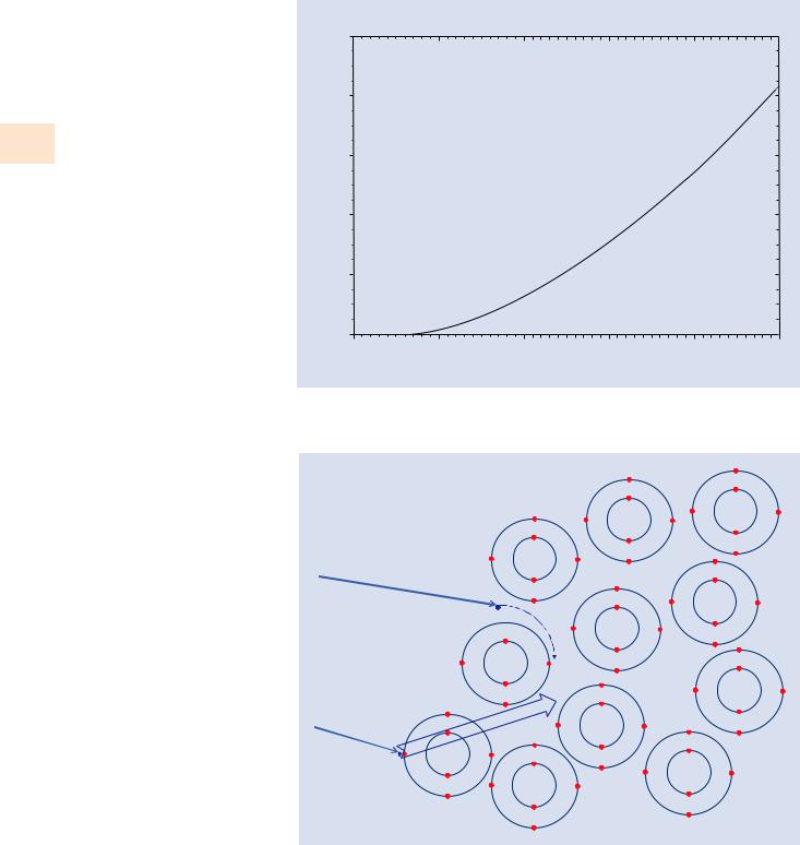
where ip is the beam current, and n is a constant depending on the particular element and shell (Lifshin et al. 1980). The value of n is typically in the range 1.5–2.0. Equation 4.8 is plotted for an exponent of n = 1.7 in . Fig. 4.9. The intensity

rises rapidly from a zero value at U = 1. For a reasonably efficient degree of X-ray excitation, it is desirable to select E0 so that U0 > 2 for the highest value of Ec among the elements of interest.

4.3\ X-Ray Continuum (bremsstrahlung)

Simultaneously with the inner shell ionization events that lead to characteristic X-ray emission, a second physical process operates to generate X-rays, the “braking radiation,” or bremsstrahlung, process. As illustrated in . Fig. 4.10, because of the repulsion that the beam electron experiences in the negative charge cloud of the atomic electrons, it undergoes deceleration and loses kinetic energy, which is released as a photon of electromagnetic radiation. The energy lost due to deceleration can take on any value from a slight deceleration involving the loss of a few electron volts up to the loss of the total kinetic energy carried by the beam electron in a single event. Thus, the bremsstrahlung X-rays span all energies from a practical threshold of 100 eV up to the incident beam energy, E0, which corresponds to an incident beam electron suffering total energy loss by deceleration in the Coulombic field of a surface atom as the beam electron enters the target and before it has lost any energy in any other inelastic scattering events. The braking radiation process thus forms a continuous energy spectrum, also referred to as the “X-ray continuum,” from 100 eV to E0, which is the so-called Duane–Hunt limit. The X-ray continuum forms a background beneath any characteristic X-rays produced by the atoms. The bremsstrahlung process is anisotropic, being somewhat peaked in the

4

Overvoltage, U = E0/Ec

. Fig. 4.10  Schematic illustration of the braking radiation (bremsstrahlung) process giving rise to the X-ray continuum

Eν

Eν =E0

direction of the electron travel. In thin specimens where the beam electron trajectories are nearly aligned, this anisotropy can result in a different continuum intensity in the forward direction along the beam relative to the backward direction.

However, in thick specimens, the near-randomization of the beam electron trajectory segments by elastic scattering effectively smooths out this anisotropy, so that the X-ray continuum is effectively rendered isotropic.

4.3 · X-Ray Continuum (bremsstrahlung)

4.3.1\ X-Ray Continuum Intensity

The intensity of the X-ray continuum, Icm , at an energy Eν is described by Kramers (1923) as

where ip is the incident beam current and Z is the atomic number. For a particular value of the incident energy, E0, the intensity of the continuum decreases rapidly relative to lower photon energies as Eν approaches E0, the Duane–Hunt limit.

An important parameter in electron-excited X-ray microanalysis is the ratio of the characteristic X-ray intensity to the X-ray continuum intensity at the same energy, Ech = Eν, often referred to as the “peak-to-background, P/B.” The P/B can be estimated from Eqs. (4.8) and (4.9) with the approximation that Eν ≈ Ec so that Eq. (4.9) can be rewritten as—

Taking the ratio of Eqs. (4.8) and (4.10) gives

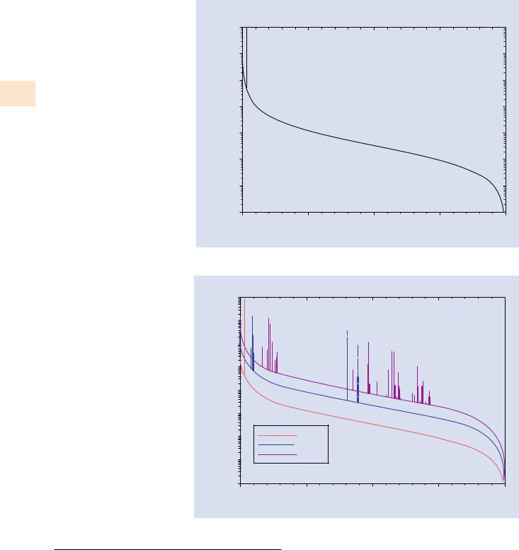
The P/B is plotted in . Fig. 4.11 with the assumption that n = 1.7, where it is seen that at low overvoltages, which are often used in electron-excited X-ray microanalysis, the characteristic intensity is low relative to higher values of U, and the intensity rises rapidly with U, while the P/B increases rapidly at low overvoltage but then more slowly as the overvoltage increases.

4.3.2\ The Electron-Excited X-Ray Spectrum,

As-Generated

The electron-excited X-ray spectrum generated within the target thus consists of characteristic and continuum X-rays and is shown for pure carbon with E0 =20 keV in . Fig. 4.12, as calculated with the spectrum simulator in NIST Desktop Spectrum Analyzer (Fiori et al. 1992), using the Pouchou and Pichoir expression for the K-shell ionization cross section and the Kramers expression for the continuum intensity (Pouchou and Pichoir 1991; Kramers 1923). Because of the energy dependence of the continuum given by Eq. 4.10, the generated X-ray continuum has its highest intensity at the lowest photon energy and decreases at higher photon energies, reaching zero intensity at E0. By comparison, the energy span of the characteristic C–K peak is its natural width of only 1.6 eV, which is related to the lifetime of the excited K-shell vacancy. The energy width for K-shell emission up to 25 keV photon energy is shown in . Fig. 4.2 (Krause and Oliver 1979). For photon energies below 25 keV, the characteristic X-ray peaks from the K-, L-, and M- shells have natural widths less than 10 eV. In the calculated spectrum of . Fig. 4.12, the C–K peak is therefore plotted as a narrow line. (X-ray peaks are often referred to as “lines” in the literature, a result of their appearance in highenergy resolution measurements of X-ray spectra by diffrac- tion-based X-ray spectrometers.) The X-ray spectra as-generated in the target for carbon, copper, and gold are compared in . Fig. 4.13, where it can be seen that at all photon energies the intensity of the X-ray continuum increases with Z, as given by Eq. 4.9. The increased complexity of the characteristic X-rays at higher Z is also readily apparent.

. Fig. 4.11  X-ray intensity emitted from a thick specimen and P/B, both as a function of overvoltage with exponent n = 1.7

8

6

2

0

1.0

Relative X-ray intensity and P/B (thick specimen)

P/B

Relative X-ray intensity

As-generated electron-excited X-ray spectrum of carbon

As-generated electron-excited X-ray spectra

C

Cu

Au

4.3.3\ Range of X-ray Production

As the beam electrons scatter inelastically within the target and lose energy, inner shell ionization events can be produced from U0 down to U = 1, so that depending on E0 and the value(s) of Ec represented by the various elements in the target, X-rays will be generated over a substantial portion of the interaction volume. The “X-ray range,” a

crude estimate of the limiting range of X-ray generation, can be obtained from a simple modification of the Kanaya–Okayama range equation (IV-5) to compensate for the portion of the electron range beyond which the energy of beam electrons has deceased below a specific value of Ec:

4.3 · X-Ray Continuum (bremsstrahlung)

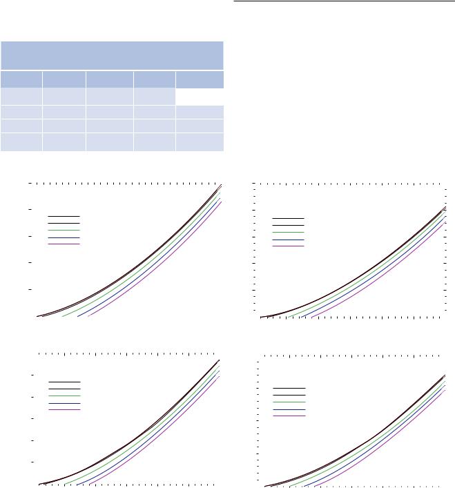
. Table 4.2 lists calculations of the range of generation for copper K-shell X-rays (Ec = 8.98 keV) produced in various host elements, for example, a situation in which copper is present at a low level so it has a negligible effect on the overall Kanaya–Okayama range. As the incident beam energy decreases to E0 = 10 keV, the range of production of copper K-shell X-rays decreases to a few hundred nanometers because of the very low overvoltage, U0 = 1.11. The X-ray range

. Table 4.2  Range of Cu K-shell (Ec = 8.98 keV) X-ray

generation in various matrices

Beam energy (keV)

in various matrices for the generation of various characteristic X-rays spanning a wide range of Ec is shown in . Fig. 4.14a–d.

4.3.4\ Monte Carlo Simulation of X-Ray

Generation

The X-ray range given by Eq. 4.12 provides a single value that captures the limit of the X-ray production but gives no information on the complex distribution of X-ray production within the interaction volume. Monte Carlo electron simulation can provide that level of detail (e.g., Drouin et al., 2007; Joy, 2006; Ritchie, 2015), as shown in . Fig. 4.15a, where the electron trajectories and the associated emitted photons of Cu K-L3 are shown superimposed. For example, the limit of production of Cu K-L3 that occurs when energy loss causes the beam electron energy to fall below the Cu K-shell excitation energy (8.98 keV) can be seen in the electron trajectories (green) that extend beyond the region of X-ray production (red). The effects of the host element on the

. Fig. 4.14  a X-ray range as a function of E0 for generation of K-shell X-rays of C, Al, Ti, Fe, and Cu in a C matrix. b X-ray range as a function of E0 for generation of K-shell X-rays of C, Al, Ti, Fe, and Cu in an Al matrix.

c X-ray range as a function of E0 for generation of K-shell X-rays of C, Al, Ti, Fe, and Cu in a Cu matrix. d X-ray range as a function of E0 for generation of K-shell X-rays of C, Al, Ti, Fe, and Cu in an Au matrix

52\ Chapter 4 · X-Rays

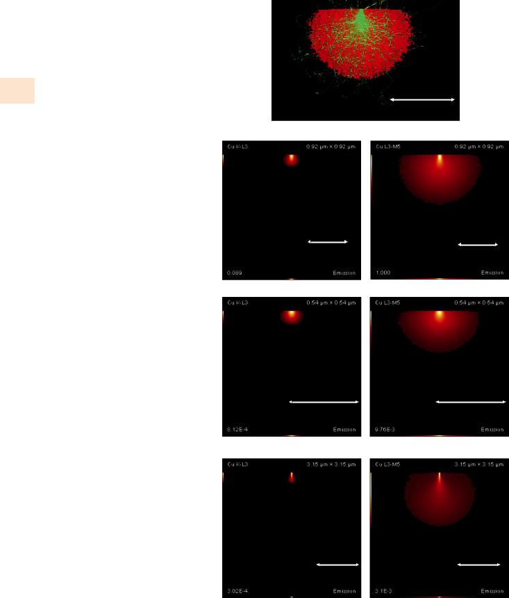
. Fig. 4.15  a Monte Carlo simulation (DTSA-II) of electron trajectories and associated Cu K-shell X-ray generation in pure copper; E0 = 20 keV.

b Monte Carlo simulation (DTSA-II) of the distribution of Cu K-shell and L-shell X-rays in a Cu matrix with E0 = 10 keV showing the X-rays that escape. c Monte Carlo simulation (DTSA-II) of the distribution of Cu K-shell and L-shell X-rays that escape in Au-1 % Cu with E0 = 10 keV. d Monte Carlo simula-

4 tion (DTSA-II) of the distribution of Cu K-shell and L-shell X-rays that escape in C-1 % Cu with E0 = 10 keV (Ritchie 2015)

a

4.3 · X-Ray Continuum (bremsstrahlung)

emission volumes for Cu K-shell and L-shell X-ray generation in three different matrices—C, Cu, and Au—is shown in

. Fig. 4.15a–c using DTSA-II (Ritchie 2015). The individual maps of X-ray production show the intense zone of X-ray generation starting at and continuing below the beam impact point and the extended region of gradually diminishing X-ray generation. In all three matrices, there is a large difference in the generation volume for the Cu K-shell and Cu L-shell X-rays as a result of the large difference in overvoltage at E0 = 10 keV: CuK U0 = 1.11 and CuL U0 = 10.8.

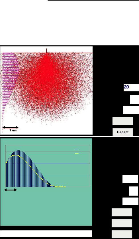
4.3.5\ X-ray Depth Distribution Function,

ϕ(ρz)

The distribution of characteristic X-ray production as a function of depth, designated “ϕ(ρz)” in the literature of quantitative electron-excited X-ray microanalysis, is a critical parameter that forms the basis for calculating the compositionally dependent correction (“A” factor) for the loss of X-rays due to photoelectric absorption. As shown in . Fig. 4.16 for Si with E0 =20 keV, Monte Carlo electron trajectory simulation provides a

. Fig. 4.16  a Monte Carlo calculation of the interaction volume and X-ray production in Si with E0 = 20 keV. The histogram construction of the X-ray depth distribution ϕ(ρz) is illustrated. (Joy Monte Carlo simulation). b ϕ(ρz) distribution of generated Si K-L3 X-rays in Si with E0 = 20 keV, and the effect of absorption from each layer, giving the fraction,

f(χ)depth, that escapes from each layer. The cumulative escape from

all layers is f(χ) = 0.80. (Joy Monte Carlo simulation) (Joy 2006)

a

Tilt/TOA 0

Number 5000

Select

Si

b

Phiroz

f(chi)